Aim: Solving the steady and unsteady 2D heat conduction problem.

Solve the 2D heat conduction equation by using the point iterative techniques Jacobi, Gauss Seidel and SOR. The Boundary conditions for the problem are as follows;

Top Boundary = 600 K,Bottom Boundary = 900 K,Left Boundary = 400 K,Right Boundary = 800 K

1)You will implement the above iterative methods for solving implicit equations with absolute error criteria is 1e-4

2. You will write code for both implicit and explicit schemes (This is for the Transient Analysis only)

Objectives of the report

1. Steady State
2. Unsteady State (Transient)
3. Matlab Script
   • Steady State
   • Implicit and Explicit Methods
4. Results

A) Steady State

• The heat conduction equation is given as

`(∂^2 T)/(∂x^2) +(∂^2 T)/(∂y^2 )=1/α (∂T)/(∂t)`

• We solve the steady state form numerically where `(∂T)/(∂t)=0` by converting to its algebraic form via discretisation

`(T_(i+1,j)-2T_(i,j)+T_(i-1,j))/(∆x^2) +(T_(i,j+1)-2T_(i,j)+T_(i,j-1))/(∆y^2) =0`

• In the case of dx=dy and re-arranging to give `T_(i,j)` as

`T_(i,j)=1/4(T_(i+1,j)+T_(i-1,j)+T_(i,j+1)+T_(i,j-1))`

This can be solved using 3 methods: Jacobi, Gauss Seidel and Successive Over relaxation (SOR). These iterative methods are used for solving linear systems of the form `Ax=b` by guessing an initial value to the solution and then terminating when `abs(b-Ax) < err` where err is the error target.

Jacobi Method

• The Jacobi method calculates an approximate solution at each grid point based on the average of the previous solution of the 4 surrounding grid points.
• The convergence rate of this method can be unacceptably slow because it does not make use of the latest grid point information available.

Gauss Seidel Method

• The GS method remedies this by taking each component of the solution as soon as it has been computed. This is achieved by replacing Told with T at the relevant grid point as shown in the script.
• Rate of convergence is higher compared to the Jacobi method.

Successive Over-Relaxation

• This method adopts the GS method in which its rate of convergence can be accelerated by using a “relaxation” parameter `ω`
• `ω>1` implies over relaxation, `ω<1` implies under-relaxation and `ω=1` implies the GS method
• Choice of `ω` can be difficult for optimal rate of convergence.

B) Unsteady State (Transient)

Explicit

• In these conditions for the explicit method, the approximate solution to the heat equation requires the consideration of the temporal component `(∂T)/(∂t)≠0`
• This can be solved numerically via 2 methods, namely the explicit and implicit method.
• The explicit method can be considered as a type of time marching solution where the unknown quantity is written explicitly in terms of the known quantities.
• Hence iterative methods need not be incorporated with this time marching scheme.
• We adopt the 2^nd order central difference scheme for the spatial component of the solution and a 1^st order forward difference scheme for the temporal component.
• Replacing the above analytical expression with their associated schemes we arrive at

`1/α (T_(i,j)^(n+1)-T_(i,j)^n)/(∆t)=(T_(i+1,j)-2T_(i,j)+T_(i-1,j))/(∆x^2) +(T_(i,j+1)-2T_(i,j)+T_(i,j-1))/(∆y^2)`

• Since this is a time marching method, we can re-arrange the above equation to write `T_(i,j)^(n+1)` explicitly in terms of the remaining terms noting that these are quantities at a current time step n

Where k1 and k2 are `α(∆t)/(∆x^2)`and `α(∆t)/(∆y^2)`respectively.

• The CFL criterion below must be considered in the case of explicit methods to ensure a good balance between solution accuracy and stability.

`α(∆t)/(∆x^2) +α(∆t)/(∆y^2) ≤1`

• Ideally, the CFL should close to 1 for best accuracy but can be difficult to achieve due to stability problems.

Implicit

• For the implicit method, the quantity of interest that we must solve for appears on both sides of the difference equation and so we must adopt iterative methods to yield a solution.
• The same iterative methods as detailed previously can be deployed here.
• We consider the same schemes to represent the approximate solution as shown below.

`T_(i,j)^(n+1)=T_(i,j)^n+k1(T_(i+1,j)-2T_(i,j)+T_(i-1,j))+k2(T_(i,j+1)-2T_(i,j)+T_(i,j-1))`

• The crucial difference here is that the quantity of interest to be iteratively solved for at `n+1`appears on both sides of the equation because the terms in the brackets are at grid points for n+1
• Thus, after some re-arrangement, we arrive at

`T_(i,j)^(n+1)=(T_(i,j)^n)/(1+2k1+2k2)+(k1(T_(i+1,j)+T_(i-1,j)))/(1+2k1+2k2)+(k2(T_(i,j+1)+T_(i,j-1)))/(1+2k1+2k2)`

• This is then solve using the iterative methods detailed in the steady state section.

C) Maltlab Script

The following function script contains all the solvers along their unique parameters. Some of the inputs are defined via global variables.

function output=solvers(iter_solver)

global L nx T_t T_b T_l T_r omega tol error

%inputs

% L=1;

% nx=10;

ny=nx;

T=ones(nx,ny);

%assigning BC's

T(:,1)=T_l;

T(:,end)=T_r;

T(1,:)=T_t;

T(end,:)=T_b;

%create copy of u

Told=T;

x=linspace(0,L,nx);

y=linspace(0,L,ny);

dx=L/(nx-1);

dy=L/(ny-1);

alpha=0.1;

t=0.01;

dt=0.01;

nt=t/dt;

k1=alpha*dt/dx^2;

k2=alpha*dt/dy^2;

term1=(1+2*k1+2*k2)^(-1);

term2=k1*term1;

term3=k2*term1;

Tprev=Told;

CFL=alpha*dt/dx^2;

%for setting up contour plots

[~,~]=meshgrid(x,y);

• For the Jacobi method we assign a double loop calculation to solve for the unknown data on the grid points in x and y direction.
• This is placed inside a while loop until the actual error is less than the predefined target error.
• We use counter and tictoc functions to output the number of iterations and simulation time respectively via the sprintf function.
• A similar approach is adopted for the GS and SOR methods with the exception that the difference equations are modified accordingly as described previously.

%jacobi method

if iter_solver==1

cntr=1;

tic

while(error > tol)

for i=2:nx-1

for j=2:ny-1

T(i,j)=0.25*((Told(i+1,j)+Told(i-1,j))+...

(Told(i,j+1)+Told(i,j-1)));

end

end

error=max(max(abs(Told-T)));

%to ensure using new value of u and not old value

%and to update the velocity after the error calculation

Told=T;

%increment the counter

cntr=cntr+1;

figure(1)

[~,~]=contourf(x,y,T,'ShowText','on');

colormap(jet);

colorbar;

xlabel('X axis');

ylabel('Y axis');

pause(0.03)

end

txt1=sprintf('Iteration numer=%d',cntr);

txt2=sprintf('Sim Time=%d',toc);

title({'Steady State-Jac',txt1,txt2});

toc

end

• For the implicit Jacobi method, we place the spatial iteration loop inside a time loop to account for the additional temporal component of the heat equation.
• The difference equations are modified accordingly.
• The same approach is used for the other 2 iterative methods in the implicit only schemes.

% Implicit Transient Jacobi method

cntr=1;

tic

while(error > tol)

for k=1:nt

for i=2:nx-1

for j=2:ny-1

T(i,j)=Tprev(i,j)*term1+...

term2*(Told(i+1,j)+Told(i-1,j))+...

term3*(Told(i,j+1)+Told(i,j-1));

end

end

error=max(max(abs(Told-T)));

cntr=cntr+1;

Told=T;

figure(4)

[~,~]=contourf(x,y,T,'ShowText','on');

colormap(jet);

colorbar;

xlabel('X axis');

ylabel('Y axis');

pause(0.03)

end

Tprev=T;

end

txt1=sprintf('Iteration numer=%d',cntr);

txt2=sprintf('Sim Time=%d',toc);

title({'Transient Implicit Jacobi',txt1,txt2});

toc

• For the explicit scheme, only the spatial iteration loop is placed inside a time loop with no iteration techniques involved because the variable to be solved for is defined explicitly.

% Explicit

while(error > tol)

for k=1:nt

for i=2:nx-1

for j=2:ny-1

T(i,j)=Told(i,j)+...

k1*(Told(i+1,j)-2*Told(i,j)+Told(i-1,j))+...

k2*(Told(i,j+1)-2*Told(i,j)+Told(i,j-1));

end

end

D) Results

• The following plots shows the output for each of the solvers as detailed previously.
• The contours show for a given temperature BC on all sides of the square, how the temperature at interior points can be evaluated by the “mean value principle”
• This principle states
  • that the temperature at equilibrium of a given point in a body is equal to the average temperature of the nearby points.
• It is shown that the different techniques yield the same solution albeit with different simulation times and iterations of which will be discussed in the next report.

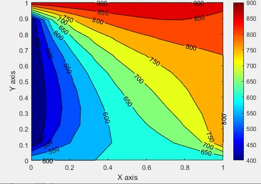
Figure 1 Steady State Jacobi

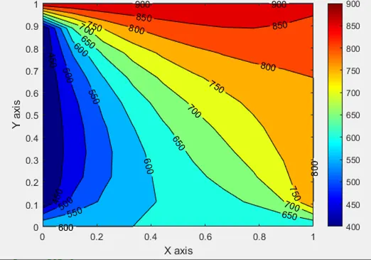
Figure 2 Steady State GS

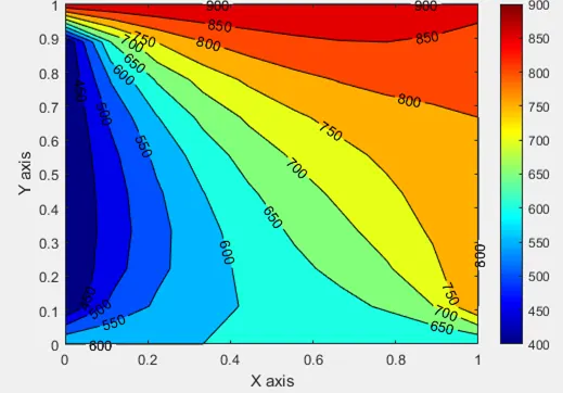
Figure 3 Steady State SOR

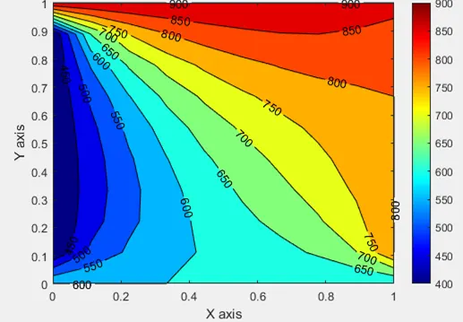
Figure 4 Transient Implicit Jacobi

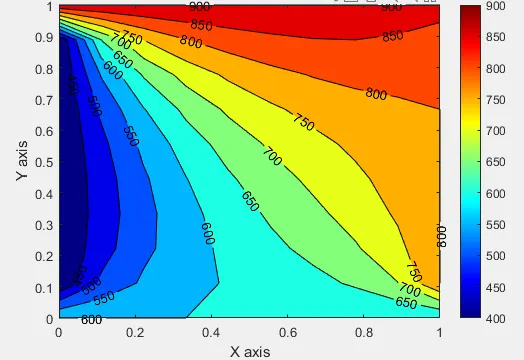
Figure 5 Transient Implicit GS

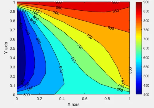
Figure 6 Transient Implicit SOR

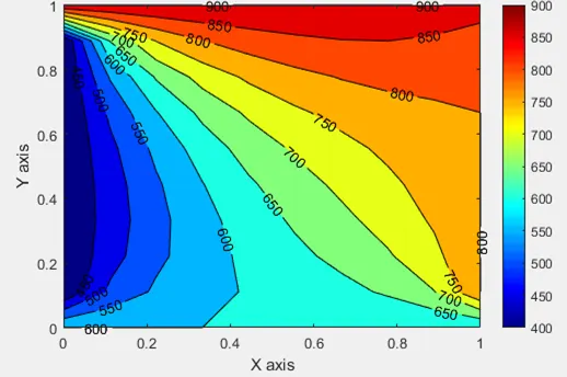
Figure 7 Transient Explicit

function output=solvers(iter_solver)
global L nx T_t T_b T_l T_r omega tol error
%inputs
% L=1;
% nx=10;
ny=nx;
T=ones(nx,ny);
%assigning BC's
T(:,1)=T_l;
T(:,end)=T_r;
T(1,:)=T_t;
T(end,:)=T_b;
%create copy of u
Told=T;
x=linspace(0,L,nx);
y=linspace(0,L,ny);
dx=L/(nx-1);
dy=L/(ny-1);
alpha=0.3;
t=0.01;
dt=0.01;
nt=t/dt;
k1=alpha*dt/dx^2;
k2=alpha*dt/dy^2;
term1=(1+2*k1+2*k2)^(-1);
term2=k1*term1;
term3=k2*term1;
Tprev=Told;
CFL=alpha*dt/dx^2
%for setting up contour plots
[~,~]=meshgrid(x,y);

%jacobi method

if iter_solver==1
	cntr=1;
         tic
 	     while(error > tol)
			for i=2:nx-1
				for j=2:ny-1
					T(i,j)=0.25*((Told(i+1,j)+Told(i-1,j))+...
                                (Told(i,j+1)+Told(i,j-1)));
				end
			end
			error=max(max(abs(Told-T)));
			%to ensure using new value of u and not old value
			%and to update the velocity after the error calculation
			Told=T;
			%increment the counter
			cntr=cntr+1;
            figure(1)
            [~,~]=contourf(x,y,T,'ShowText','on');
            colormap(jet);
            colorbar;
			xlabel('X axis');
			ylabel('Y axis');
			pause(0.03)

	
		
        end
        txt1=sprintf('Iteration numer=%d',cntr);
        txt2=sprintf('Sim Time=%d',toc);
        title({'Steady State-Jac',txt1,txt2});
        toc
        
end


%GS method
if iter_solver==2
	cntr=1;
         tic
 	     while(error > tol)
			for i=2:nx-1
				for j=2:ny-1
					T(i,j)=0.25*(T(i-1,j)+Told(i+1,j)+...
                                (Told(i,j+1)+T(i,j-1)));
				end
			end
			error=max(max(abs(Told-T)));
			%to ensure using new value of u and not old value
			%and to update the velocity after the error calculation
			Told=T;
			%increment the counter
			cntr=cntr+1;
            figure(2)
            [~,~]=contourf(x,y,T,'ShowText','on');
            colormap(jet);
            colorbar;
			xlabel('X axis');
			ylabel('Y axis');
			pause(0.03)

	
		
        end
        txt1=sprintf('Iteration numer=%d',cntr);
        txt2=sprintf('Sim Time=%d',toc);
        title({'Steady State-GS',txt1,txt2});
        toc
end

%SOR method
if iter_solver==3
	cntr=1;  
          tic
          while(error > tol)
			for i=2:nx-1
				for j=2:ny-1
					T(i,j)=(1-omega)*Told(i,j)+...
                            omega*(0.25*(T(i-1,j)+Told(i+1,j)+...
                                         Told(i,j+1)+T(i,j-1)));
				end
			end
			error=max(max(abs(Told-T)));
			%to ensure using new value of u and not old value
			%and to update the velocity after the error calculation
			Told=T;
			%increment the counter
			cntr=cntr+1;
            figure(3)
			[~,~]=contourf(x,y,T,'ShowText','on');
            colormap(jet);
            colorbar;
			xlabel('X axis');
			ylabel('Y axis');
			pause(0.03)

	
		
         end
         txt1=sprintf('Iteration numer=%d',cntr);
         txt2=sprintf('Sim Time=%d',toc);
         title({'Steady State-SOR',txt1,txt2});
         toc
end

% Implicit Transient Jacobi method
if iter_solver==4
	cntr=1; 
         tic
	     while(error > tol)
            for k=1:nt
                for i=2:nx-1
                    for j=2:ny-1
                        T(i,j)=Tprev(i,j)*term1+...
                               term2*(Told(i+1,j)+Told(i-1,j))+...
                               term3*(Told(i,j+1)+Told(i,j-1));
                    end
                end
                
            error=max(max(abs(Told-T)));
			cntr=cntr+1;
            Told=T; 
            
          
            figure(4)
            [~,~]=contourf(x,y,T,'ShowText','on');
            colormap(jet);
            colorbar;
            xlabel('X axis');
            ylabel('Y axis');
            pause(0.03)

            
            end   
            Tprev=T;
       end
       txt1=sprintf('Iteration numer=%d',cntr);
       txt2=sprintf('Sim Time=%d',toc);
       title({'Transient Implicit Jacobi',txt1,txt2});
       toc
end

%Implicit Transient GS method
if iter_solver==5
	cntr=1; 
        tic
		while(error > tol)
            for k=1:nt
                for i=2:nx-1
                    for j=2:ny-1
                        T(i,j)=Tprev(i,j)*term1+...
                               term2*(Told(i+1,j)+T(i-1,j))+...
                               term3*(Told(i,j+1)+T(i,j-1));
                    end
                end
			error=max(max(abs(Told-T)));
			cntr=cntr+1;
            Told=T; 
            
            %increment the counter
            figure(5)
            [~,~]=contourf(x,y,T,'ShowText','on');
            colormap(jet);
            colorbar;
            xlabel('X axis');
            ylabel('Y axis');
            pause(0.03)

            
            end   
            Tprev=T;
        end 
        txt1=sprintf('Iteration numer=%d',cntr);
        txt2=sprintf('Sim Time=%d',toc);
        title({'Transient Implicit GS',txt1 txt2});
        toc
end

%Implicit Transient SOR method
if iter_solver==6
	cntr=1;   
        tic
		while(error > tol)
            for k=1:nt
                for i=2:nx-1
                    for j=2:ny-1
                        T(i,j)= term1*Tprev(i,j)+...
                                term2*((1-omega)*Told(i-1,j)+omega*T(i-1,j)+Told(i+1,j))+...
                                term3*((1-omega)*Told(i,j-1)+omega*T(i,j-1)+Told(i,j+1));
                    end
                end
			error=max(max(abs(Told-T)));
			cntr=cntr+1;
            Told=T; 
            
            %increment the counter
            figure(6)
            [~,~]=contourf(x,y,T,'ShowText','on');
            colormap(jet);
            colorbar;
            xlabel('X axis');
            ylabel('Y axis');
            pause(0.03)

            
            end   
            Tprev=T;
        end 
        txt1=sprintf('Iteration numer=%d',cntr);
        txt2=sprintf('Sim Time=%d',toc);
        title({'Transient Implicit SOR',txt1 txt2});
        toc
end


% Explicit
if iter_solver==7
	cntr=1; 
        tic
		while(error > tol)
            for k=1:nt
                for i=2:nx-1
                    for j=2:ny-1
                        T(i,j)=Told(i,j)+...
                               k1*(Told(i+1,j)-2*Told(i,j)+Told(i-1,j))+...
                               k2*(Told(i,j+1)-2*Told(i,j)+Told(i,j-1));
                    end
                end
                
            error=max(max(abs(Told-T)));
			cntr=cntr+1;
            Told=T; 
            
          
            figure(7)
            [~,~]=contourf(x,y,T,'ShowText','on');
            colormap(jet);
            colorbar;
            xlabel('X axis');
            ylabel('Y axis');
            pause(0.03)
            
            end   
          
        end 
        txt1=sprintf('Iteration numer=%d',cntr);
        txt2=sprintf('CFL=%d',CFL);
        txt3=sprintf('Sim Time=%d',toc);
        title({'Transient Explicit',txt1,txt2 txt3});
        toc
end
output=[];
end

clear all
close all
clc

global L nx T_t T_b T_l T_r omega tol error

L=1;
nx =10;
T_t=600;
T_b=900;
T_l=400;
T_r=800;

%SOLVER CHOICE
%%%%%%%%%%%%%%%%%%%%%%%%%%%%%%%%%%%%%%%%%%%%%%%%%%%%%%%%%%%%%
%Steady State 
%             Jacobi 1, Steady State GS 2   State State SOR 3
%%%%%%%%%%%%%%%%%%%%%%%%%%%%%%%%%%%%%%%%%%%%%%%%%%%%%%%%%%%%%
%Transient 
%    Implicit Jacobi 4,     Implicit GS 5      Implicit SOR 6
%    Explicit        7
%%%%%%%%%%%%%%%%%%%%%%%%%%%%%%%%%%%%%%%%%%%%%%%%%%%%%%%%%%%%%
%Select solver 
iter_solver=7;
error=100;
tol=1e-4;

%SOR parameter
omega=1.8;

output=solvers(iter_solver);