Week 7 - Simulation of a 1D Super-sonic nozzle flow simulation using Macormack Method
%% NON CONSERVATIVE
clc;
clear;
close all

n=31;
x=linspace(0,3,n);
dx = x(2)-x(1);
gamma = 1.4;
% calc. initial profiles

rho = 1-0.3146*x;
T = 1-0.2314*x;
v = (0.1+1.09*x).*T.^0.5;
a = 1+2.2*(x-1.5).^2;

% Time steps
nt = 100;
dt = 0.01;

for k=1:nt

  rho_old = rho;
  v_old = v;
  T_old = T;

  % PRedictor step
  for j=2:n-1
    dvdx = (v(j+1)-v(j))/dx;
    drhodx = (rho(j+1)-rho(j))/dx;
    dTdx = (T(j+1)-T(j))/dx;
    dlogadx = (log(a(j+1))-log(a(j)))/dx;

    % continuity eauation
    drhodt_p(j) = -rho(j)*dvdx - rho(j)*v(j)*dlogadx - v(j)*drhodx;

    % Momentum equation
    dvdt_p(j) = -v(j)*dvdx - (1/gamma)*(dTdx + (T(j)/rho(j))*drhodx);

    % Energy equation
    dTdt_p(j) = -v(j)*dTdx - (gamma-1)*T(j)*(dvdx+v(j)*dlogadx);

    % Solution update
    rho(j) = rho(j)+drhodt_p(j)*dt;
    v(j) = v(j)+ dvdt_p(j)*dt;
    T(j) = T(j) + dTdt_p(j)*dt;
  endfor

  % Corrector step
  for j=2:n-1
    dvdx = (v(j)-v(j-1))/dx;
    drhodx = (rho(j)-rho(j-1))/dx;
    dTdx = (T(j)-T(j-1))/dx;
    dlogadx = (log(a(j))-log(a(j-1)))/dx;

    % continuity equation
    drhodt_c(j) = -rho(j)*dvdx - rho(j)*v(j)*dlogadx - v(j)*drhodx;

    % Momentum equation
    dvdt_c(j) = -v(j)*dvdx - (1/gamma)*(dTdx + (T(j)/rho(j))*drhodx);

    % Energy equation
    dTdt_c(j) = -v(j)*dTdx - (gamma-1)*T(j)*(dvdx+v(j)*dlogadx);
   endfor

  % compute the average time derivative

  drhodt = 0.5*(drhodt_p+drhodt_c);
  dvdt = 0.5*(dvdt_p+dvdt_c);
  dTdt = 0.5*(dTdt_p + dTdt_c);

  % Final solution update
    for j=1:n-1
    rho(j) = rho_old(j)+drhodt(j)*dt;
    v(j) = v_old(j)+ dvdt(j)*dt;
    T(j) = T_old(j) + dTdt(j)*dt;
    endfor

% Apply the boundary conditions
v(1) = 2*v(2) - v(3);

% outlet
v(n) = 2*v(n-1) - v(n-2);
rho(n) = 2*rho(n-1)- rho(n-2);
T(n) = 2*T(n-1) - T(n-2);

subplot(3,1,1)

plot(x,v)
title('v')
grid on
grid minor
pause(0.0003)

subplot(3,1,2)

plot(x,rho)
title('rho')
grid on
grid minor
pause(0.0003)

subplot(3,1,3)

plot(x,T)
title('T')
xlabel('x')
grid on
grid minor
pause(0.0003)

endfor
%% CONSERVATIVE

clc;
clear;
close all

n=31;
x=linspace(0,3,n);
dx = x(2)-x(1);
gamma = 1.4;
% calc. initial profiles

a = 1+2.2*(x-1.5).^2;
RHO(1:length(a))=0;
TT(1:length(a))=0;
RHO(x<=0.5) =1;
RHO(x>0.50000 & x<=1.50000) = 1-0.366*(x(x>0.50000 & x<=1.50000)-0.50000);
RHO(x>1.50000 & x<=30000) = 0.634-0.3879*(x(x>1.50000 & x<=3.0000)-1.5);
TT(x<=0.50000) = 1;
TT(x>0.50000 & x<=1.50000) = 1 - 0.167*(x(x>0.50000 & x<=1.50000)-0.50000);
TT(x>1.50000 & x<=30000) = 0.833-0.3507*(x(x>1.50000 & x<=30000)-1.50000);
aa = a(1)/5.95; #non-dimenisionalized area, a=1 and normalizing area =1/5.95 = 0.1681
A=a/aa;

U1 = RHO.*A;
U2=ones(1,length(x))*0.59; # assuming uniform flow rate through out the nozzle
V = U2./U1;
U3 = U1.*(TT/(gamma-1) + gamma*(V.^2)/2);

##F1 = U2;
##F2 = (U2.^2)./U1 +((gamma-1)/gamma)*(U3-(gamma/2)*((U2.^2)./U1));
##F3 = (gamma*(U2.*U3)./U1 - gamma*(gamma-1)*(U2.^3)./(2*U1.^2));
##J2 = (1/gamma)*RHO(1:length(x)-1).*TT(1:length(x)-1).*(diff(A)./diff(x));
% Time steps
nt = 100;
##dt = 0.01;
C = 0.5; # courant number
Tref = 20;
for k=1:nt
  F1 = U2;
  F2 = (U2.^2)./U1 +((gamma-1)/gamma)*(U3-(gamma/2)*((U2.^2)./U1));
  F3 = (gamma*(U2.*U3)./U1 - gamma*(gamma-1)*(U2.^3)./(2*U1.^2));
  J2 = (1/gamma)*RHO(1:length(x)-1).*TT(1:length(x)-1).*(diff(A)./diff(x));
  c_air   = (331.3+0.606*(TT*Tref))/(331.3+0.606*(Tref));
##c_air = ((303/273)^0.5);
  dt      = min(C*(dx)./(c_air(1:end-1)+V(1:end-1)));
  Dt(k)   = dt;
  RHO_old = RHO;
  V_old   = V;
  TT_old  = TT;
  U1_old  = U1;
  U2_old  = U2;
  U3_old  = U3;
  % PRedictor step
  for j=2:n-1
    dF1dx = (F1(j+1)-F1(j))/dx;
    dF2dx = (F2(j+1)-F2(j))/dx;
    dF3dx = (F3(j+1)-F3(j))/dx;

    % continuity eauation
    dU1dt_p(j) = -dF1dx;

    % Momentum equation
    dU2dt_p(j) = -dF2dx+J2(j);

    % Energy equation
    dU3dt_p(j) = -dF3dx;

    % Solution update
    U1(j) = U1(j)+ dU1dt_p(j)*dt;
    U2(j) = U2(j)+ dU2dt_p(j)*dt;
    U3(j) = U3(j)+ dU3dt_p(j)*dt;

    RHO(j) = U1(j)/A(j);
    V(j)   = U2(j)/U1(j);
    TT(j)  = (gamma-1)*(U3(j)/U1(j) - (gamma/2)*(V(j))^2);
  endfor
  U1(1) = A(1);
  U2(1) = 2*U2(2)-U2(3);
  U3(1) = U1(1).*(TT(1)/(gamma-1) + gamma*(V(1).^2)/2);


  for j=1:1:n-1
    F1(j) = U2(j);
    F2(j) = (U2(j).^2)./U1(j) +((gamma-1)/gamma)*(U3(j)-(gamma/2)*((U2(j).^2)./U1(j)));
    F3(j) = (gamma*(U2(j).*U3(j))./U1(j) - gamma*(gamma-1)*(U2(j).^3)./(2*U1(j).^2));
    if j>1
    J2(j) = (1/gamma)*RHO(j).*TT(j).*((A(j)-A(j-1))/(dx));
    endif
  endfor
  % outlet
##  U1(n) = 2*U1(n-1) - U1(n-2);
##  U2(n) = 2*U2(n-1) - U2(n-2);
##  U3(n) = 2*U3(n-1) - U3(n-2);
##
##
##  F1(n) = U2(n);
##  F2(n) = (U2(n).^2)./U1(n) +((gamma-1)/gamma)*(U3(n)-(gamma/2)*((U2(n).^2)./U1(n)));
##  F3(n) = (gamma*(U2(n).*U3(n))./U1(n) - gamma*(gamma-1)*(U2(n).^3)./(2*U1(n).^2));
##  RHO(n) = U1(n)/A(n);
##  TT(n)  = (gamma-1)*(U3(n)/U1(n) - (gamma/2)*(U2(n)/U1(n))^2);
##  V(n)   = U2(n)/U1(n);
##  J2(n) = (1/gamma)*RHO(n).*TT(n).*((A(n)-A(n-1))/(x(n)-x(n-1)));
  % Corrector step
  for j=2:n-1
    dF1dx = (F1(j)-F1(j-1))/dx;
    dF2dx = (F2(j)-F2(j-1))/dx;
    dF3dx = (F3(j)-F3(j-1))/dx;

    % continuity eauation
    dU1dt_c(j) = -dF1dx;

    % Momentum equation
    dU2dt_c(j) = -dF2dx+J2(j);

    % Energy equation
    dU3dt_c(j) = -dF3dx;
   endfor

  % compute the average time derivative

  dU1dt = 0.5*(dU1dt_c+dU1dt_p);
  dU2dt = 0.5*(dU2dt_c+dU2dt_p);
  dU3dt = 0.5*(dU3dt_c+dU3dt_p);

  % Final solution update
  for j=1:n-1
    U1(j) = U1_old(j) + dU1dt(j)*dt;
    U2(j) = U2_old(j) + dU2dt(j)*dt;
    U3(j) = U3_old(j) + dU3dt(j)*dt;

    RHO(j) = U1(j)/A(j);
    TT(j)  = (gamma-1)*(U3(j)/U1(j) - (gamma/2)*(U2(j)/U1(j))^2);
    V(j)   = U2(j)/U1(j);

    RHO1(k,j) = round(RHO(j)*1000)/1000;
    TT1(k,j)  = round(TT(j)*1000)/1000;
    V1(k,j)   = round(V(j)*1000)/1000;
  endfor

% Apply the boundary conditions
U1(1) = A(1);
U2(1) = 2*U2(2)-U2(3);
U3(1) = U1(1).*(TT(1)/(gamma-1) + gamma*(V(1).^2)/2);
% outlet
U1(n) = 2*U1(n-1) - U1(n-2);
U2(n) = 2*U2(n-1) - U2(n-2);
U3(n) = 2*U3(n-1) - U3(n-2);
F1(n) = U2(n);
F2(n) = (U2(n).^2)./U1(n) +((gamma-1)/gamma)*(U3(n)-(gamma/2)*((U2(n).^2)./U1(n)));
F3(n) = (gamma*(U2(n).*U3(n))./U1(n) - gamma*(gamma-1)*(U2(n).^3)./(2*U1(n).^2));
RHO(n)= U1(n)/A(n);
TT(n) = (gamma-1)*(U3(n)/U1(n) - (gamma/2)*(U2(n)/U1(n))^2);
V(n)  = U2(n)/U1(n);
J2(n) = (1/gamma)*RHO(n).*TT(n).*((A(n)-A(n-1))/(x(n)-x(n-1)));


RHO1(k,n) = round(RHO(n)*1000)/1000;
TT1(k,n)  = round(TT(n)*1000)/1000;
V1(k,n)   = round(V(n)*1000)/1000;

figure(1)
subplot(3,1,1)
plot(x,V,'b','LineWidth',2)
title(sprintf('Time = %d | Velocity',k*dt))
grid on
grid minor

subplot(3,1,2)
plot(x,RHO,'b','LineWidth',2)
title('Density')
grid on
grid minor

subplot(3,1,3)
plot(x, TT,'b','LineWidth',2)
title('Temperature')
xlabel('x')
grid on
grid minor

pause(0.0003)

figure(2)
subplot(3,1,1)
plot(x,U1,'b','LineWidth',2)
title(sprintf('Time = %d | U1', k*dt))
grid on
grid minor

subplot(3,1,2)
plot(x,U2,'b','LineWidth',2)
title('U2')
grid on
grid minor

subplot(3,1,3)
plot(x, U3,'b','LineWidth',2)
title('U3')
xlabel('x')
grid on
grid minor

pause(0.0003)
endfor
figure(3)
plot(Dt,'b','LineWidth',2)
title('Time Step')
grid on
grid minor

figure(4)
plot(x,U2,'b','LineWidth',2)
ylim([0.4 0.7])
yticks(0.4:0.01:0.7)
grid on
Results:
Conservative:
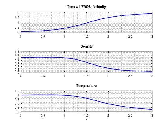
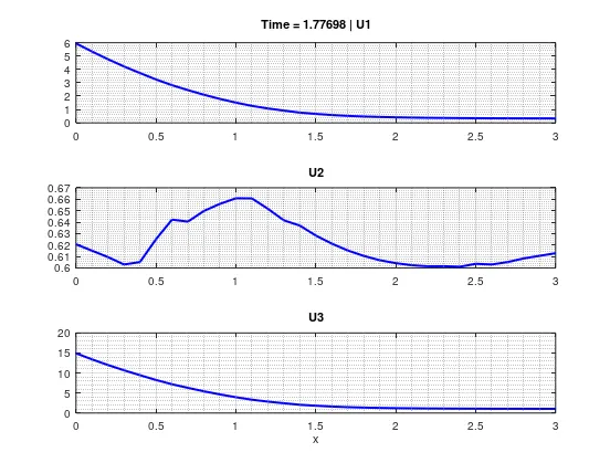
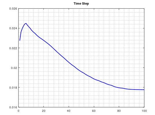
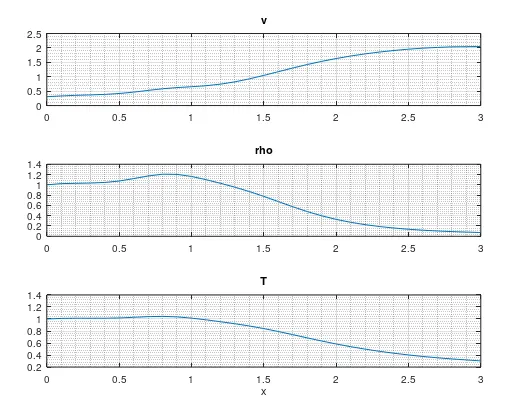
Nonconservative