Week 5 - Mid term project - Solving the steady and unsteady 2D heat conduction problem
Main Script
clc;
clear;
close all;

len_x=1; % length on first dimension
len_y=1; % length on second dimension
x=linspace(0,len_x,10);  % defining grid points in x direction
dx=x(2)-x(1);
y=linspace(0,len_y,10);% defining grid points in y direction
dy=y(2)-y(1);
[X,Y]=meshgrid(x,y); %% defining 2-d mesh
alpha=1; % constant in the conduction equation
dt=0.1; % time step
stop_time=5; % simulation time, seconds
Max_Iterations = 1000; % maximum number of iterations
iter = 1:1:Max_Iterations; % defining iteration vector
time=0:dt:stop_time; % time vector

Solver =input('Enter Solver: 1-Jacobi Transient  2-Gauss Seidal Transient  3-Jacobi SS 4-Gauss-Seidal SS:   '); % getting solver type from user

if Solver==2 || Solver ==4
Relax = input('Over Relaxation -1, No Relaxation-0:  ');
end

disp('Running simulation.....')

if Solver ==1 || Solver==2
Third_Dim = time;
% defining intial temperature grid
T(1:length(x), 1:length(y), 1:length(Third_Dim)) = 1;
T(1:length(x),1,:)=400;
T(1:length(x),end,:)=800;
T(1,1:length(y),:)=600;
T(end,1:length(y),:)=900;
Told = T;
else
Third_Dim = iter;
T(1:length(x), 1:length(y)) = 1;
T(1:length(x),1)=400;
T(1:length(x),end)=800;
T(1,1:length(y))=600;
T(end,1:length(y))=900;
Told = T;
end


%% constants in FD equtions
% transient
k1=alpha*dt/(dx^2);
k2=alpha*dt/(dy^2);
k1k2 = (1+2*k1+2*k2);
% steady state
k=2*((dx^2+dy^2)/(dx*dx*dy*dy));

tol = 1e-4; % tolerance
Error=1e9; % initial error

iter=1;
switch Solver
#Jacobi-Transient
case 1
[T, iter1, Error] = Conduction_2d_Jacobi(Told, time, x, y, tol,k1, k2, k1k2);
case 2
### Gauss-Seidal
[T, iter1, Error] = Conduction_2d_GS(Told, time, x, y, tol,k1, k2, k1k2, Relax);
## Jacobi-steady state
case 3
[T, iter1, Error] = Conduction_2d_SS_Jacobi(Told, x, y, X, Y, dx, dy, tol, k, Max_Iterations);
## Gauss-Seidal steady state
case 4
[T, iter1, Error] = Conduction_2d_SS_GS(Told, x, y, X, Y, dx,  dy, tol, k, Max_Iterations, Relax);
endswitch
disp('Simulation complete..')
if Solver == 1 || Solver ==2
Plotter(T, time, X, Y, iter1, Solver, Error)
end
Jacobi-Transient Function
function [T, iter1, Error] = Conduction_2d_Jacobi(Told, time, x, y, tol, k1, k2, k1k2)
Error=1e9;
#Jacobi
T=Told;
iter1=1;
while(Error>tol && iter1<=500)
  for t=2:1:length(time)
    for i=2:1:length(x)-1
      for j=2:1:length(y)-1
        T(i,j,t) =  (1/k1k2)*Told(i,j,t-1)+(k1/k1k2)*(Told(i-1,j,t)+Told(i+1,j,t))+(k2/k1k2)*(Told(i,j-1,t)+Told(i,j+1,t));
      end
    end
  end
Error=max(max(max(abs(T-Told))));
Told = T;
iter1 = iter1+1;
end
endfunction
Gauss-Seidal and Over-Relaxation Transient Function
function [T, iter1, Error] = Conduction_2d_GS(Told, time, x, y, tol, k1, k2, k1k2, Relax)
Error=1e9;

#Jacobi
T=Told;
Relaxation_Factor = 1.1;
iter1=1;
while(Error>tol && iter1<500)
  for t=2:1:length(time)
    for i=2:1:length(x)-1
      for j=2:1:length(y)-1
        Told1=T;
        T(i,j,t) =  (1/k1k2)*T(i,j,t-1)+(k1/k1k2)*(T(i-1,j,t)+T(i+1,j,t))+(k2/k1k2)*(T(i,j-1,t)+T(i,j+1,t));
          if Relax==1
            T = Told1+(T-Told1)*Relaxation_Factor;
          end
      end
    end
  end
Error=max(max(max(abs(T-Told))));
Told = T;
iter1 = iter1+1;

end
endfunction
Jacobi-Steady State Function
function [T, iter1, Error] = Conduction_2d_SS_Jacobi(Told, x, y, X, Y, dx, dy, tol, k, Max_Iterations)
Error=1e9;

#Jacobi
T=Told;
iter1=1;
while(Error>tol && iter1<Max_Iterations)
    for i=2:1:length(x)-1
      for j=2:1:length(y)-1
        term1 = (Told(i-1,j)+Told(i+1,j))/(dx^2);
        term2 = (Told(i,j-1)+Told(i,j+1))/(dy^2);
        T(i,j) =  (1/k)*(term1+term2);
      end
    end

Error(iter1)=max(max(abs(T-Told)));
Told = T;

contourf(X,Y,T,'ShowText','on')
set(gca,'Ydir','reverse')
xlabel('x')
ylabel('y')
Title = sprintf( 'Iteraton= %d | Error = %d', iter1, Error(iter1));
title(Title)
pause(0.003)
iter1 = iter1+1;
end
endfunction
Gauss-Seidal Steady State with Over-Relaxation
function [T, iter1, Error] = Conduction_2d_SS_GS(Told, x, y, X, Y, dx,  dy, tol, k, Max_Iterations, Relax)
Error=1e9;

#Jacobi
T=Told;
iter1=1;
Relaxation_Factor = 1.1;

while(Error>tol && iter1<Max_Iterations)
    for i=2:1:length(x)-1
      for j=2:1:length(y)-1

        Told1=T;
        term1 = (T(i-1,j)+T(i+1,j))/(dx^2);
        term2 = (T(i,j-1)+T(i,j+1))/(dy^2);
        T(i,j) =  (1/k)*(term1+term2);
         if Relax==1
            T = Told1+(T-Told1)*Relaxation_Factor;
          end
      end
    end

Error(iter1)=max(max(abs(T-Told)));
Told = T;
contourf(X,Y,T,'ShowText','on')
set(gca,'Ydir','reverse')
xlabel('x')
ylabel('y')
Title = sprintf( 'Iteraton= %d | Error = %d', iter1, Error(iter1));
title(Title)
pause(0.003)
iter1 = iter1+1;
end
endfunction
Explicit Function
function [T] = Conduction_2d_Explicit(Told, time, x, y, tol,k1, k2, k1k2)
  T=Told;
  for t=2:1:length(time)
    for i=2:1:length(x)-1
      for j=2:1:length(y)-1
        T(i,j,t) =  (1/k1k2)*T(i,j,t-1)+(k1/k1k2)*(T(i-1,j,t-1)+T(i+1,j,t-1))+(k2/k1k2)*(T(i,j-1,t-1)+T(i,j+1,t-1));
      end
    end
  end

endfunction
Plotting Function for Transinet Solvers
function [] = Plotter(T,time, X, Y, iter1, Solver, Error)

if Solver ==1 || Solver==2
  for t=1:1:length(time)
  contourf(X,Y,T(:,:,t),'ShowText','on')
  set(gca,'Ydir','reverse')
  xlabel('x')
  ylabel('y')
  Title = sprintf('Time = %d | Iteratons = %d', time(t), iter1);
  title(Title)
  pause(0.003)
  endfor
else
  for iteration=1:1:iter1
  contourf(X,Y,T(:,:,iteration),'ShowText','on')
  set(gca,'Ydir','reverse')
  xlabel('x')
  ylabel('y')
  Title = sprintf( 'Iteraton= %d | Error = %d', iteration, Error(iteration));
  title(Title)
  pause(0.003)
  endfor
end

endfunction
Results:
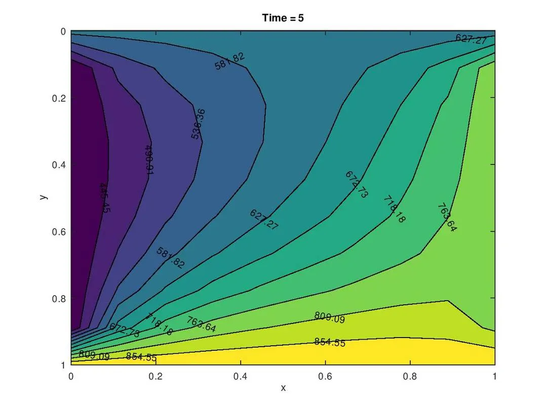
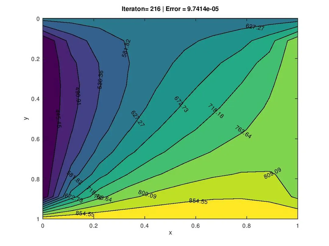
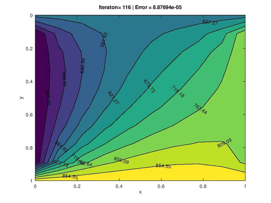
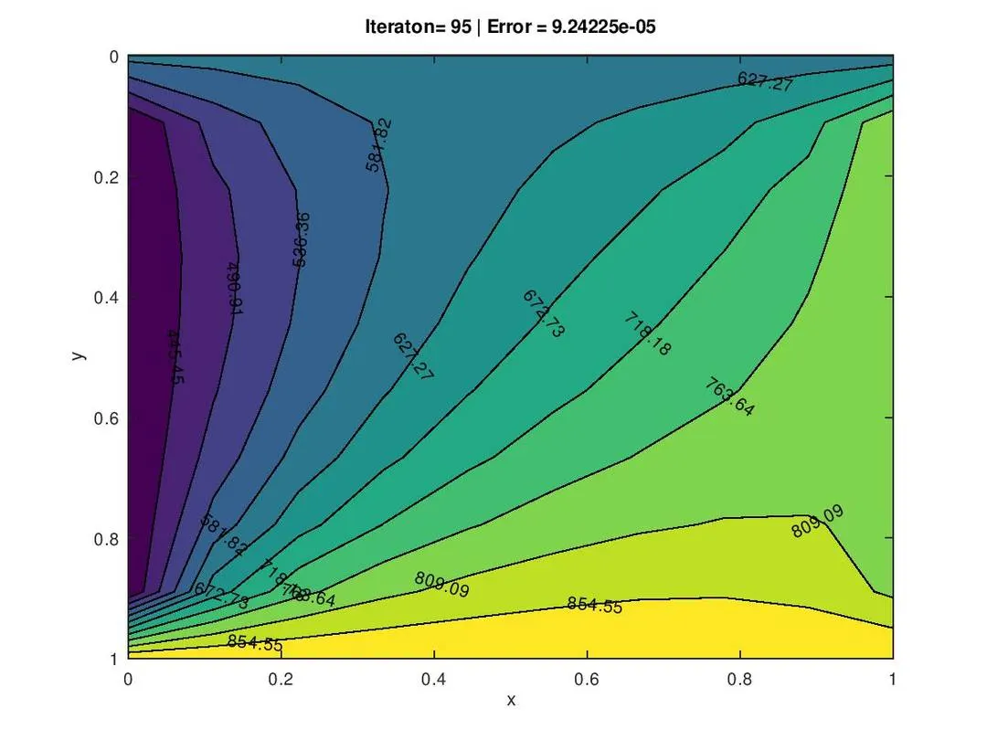
The final plot for transient and steady state cases with Jacobi, Gauss-Seidal and over relaxation are the same. Anyway, the obtained plots with iterations take for each of them is shown below. It is observed that, the trend in number of iterations taken is: Jacobi>Gauus-seidal>Over Relaxation.
The reason for this trend is that Jacobi solver updates the temperature grid only after all the points in the grid are calculated in the current iteration. But in Gauss- Seidal, the grid is updated after calculting very point in the grid in the current iteration. This means that updating is not on hold until the next iteration. With overrelaxtion, the iterations are further reduced by expditing the updating process by increasing the gain more than 1 as follows.
T = Told1+(T-Told1)*Relaxation_Factor
Plots:
Transient-Jacobi
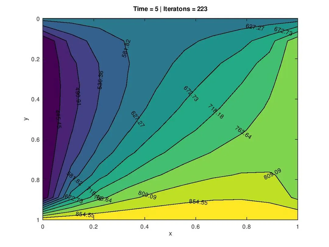
Transient Gauss Seidal
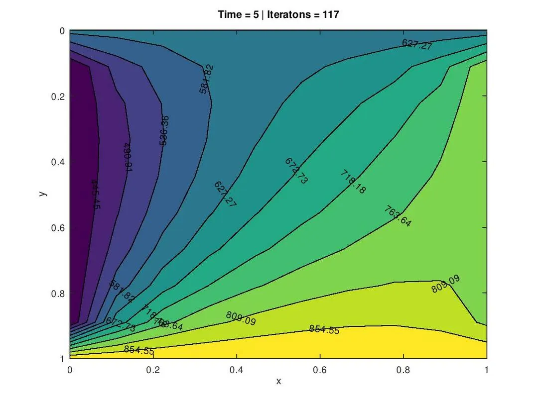
Transient Gauss Seidal with over relaxation
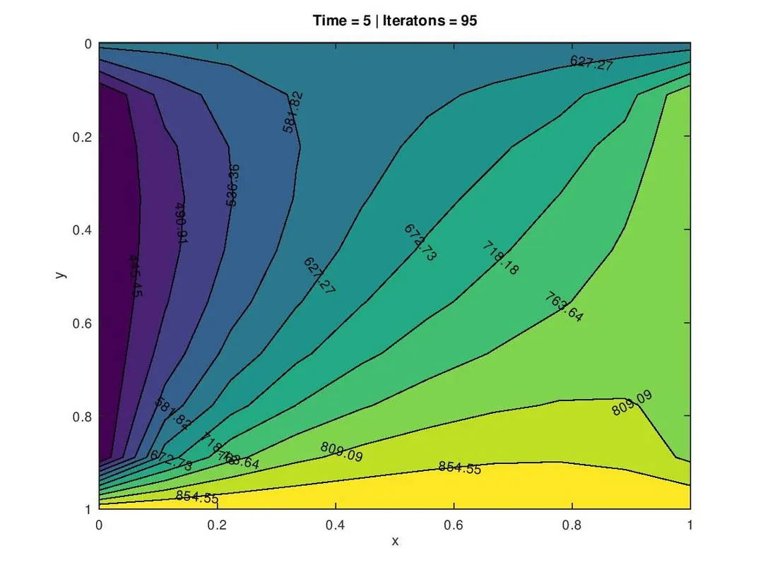
Steady state Jacobi
Steady state Gauss Seidal
Steady state Gauss Seidal with over relaxation
Explicit