Week 7 - Simulation of a 1D Super-sonic nozzle flow simulation using Macormack Method
Simulation of subsonic-supersonic isentropic nozzle flow using MacCormack’s Method
Aim:
To determine the difference between the conservative and non-conservative form of the governing equation in a CFD methodology. The objective was achieved by simulating a quasi 1D subsonic-supersonic isentropic nozzle flow using the MacCormack’s method.
Problem Definition:
In this project, we consider a steady isentrophic flow through a convergent-divergent nozzle as shown in the figure below. The flow at the inlet comes from a reservoir with pressure `p_0` and temperature `T_0`. The area of the reservoir is large and hence the inlet velocity is small. The flow expands isentrophically to supersonic speed at the nozzle exit where the pressure, temperature and velocity and Mach number are represented as `p_e`, `T_e`, `V_e` and `M_e` respectively. The flow is locally subsonic at the convergent section, sonic at the throat area and supersonic at the divergent section of the nozzle.
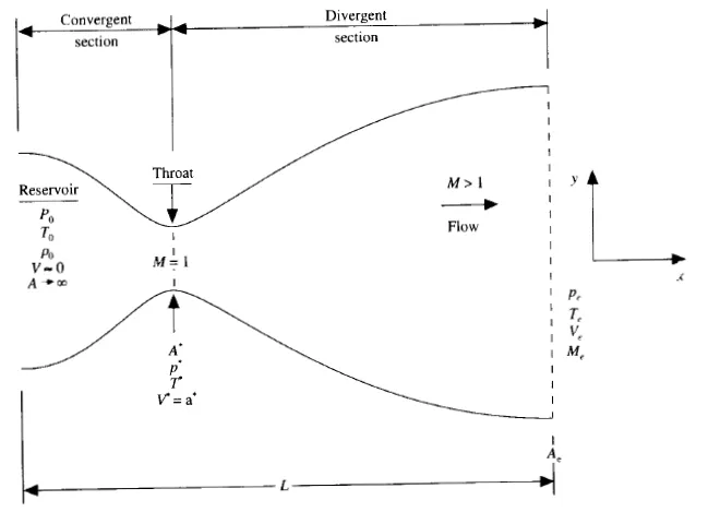
We assume a quasi 1D flow through the nozzle. It essentially means that the flow properties are assumed to vary only with x even-though in reality, the flow is 2D. Hence the governing equations for this case were derived both in conservative and non-conservative form. These equations were subsequently solved using the MacCormack’s method and the results were compared.
This problem is classic problem in gas dynamics for which analytical solutions are available. This particular problem was chosen because the numerical solutions can be compared with the analytical solutions.
Theory:
Conservation Vs Non-conservation:
The governing equations for fluid flow (mass, momentum and energy conservation) can be represented both in a conservative and non-conservative form. As an example, you can find the mass conservation equation written in both conservative and non-conservative form:
Conservative form:
`(delrho)/(delt) + nabla*(rho*V) = 0 `
Non-conservative form:
`(Drho)/(Dt) + rho*nabla*V = 0 `
Where,
`(Drho)/(Dt)` represents the total derivative
Conservative represents the conservation of a quantity in a stationary control volume and the non-conservative form represents a control volume that is moving. Theoretically, there is no difference between the two representations and they both model the fluid flow. This distinction arose out of modern CFD applications as well as a concern for when a particular form should be used for a given CFD application. The main perspective is that the conservation form of the equations can be represented by a simple generic equation, providing for numerical and programming convenience [1]. When the divergence operator is expanded, the generic equation can be represented as
` (delU)/(delt) + (delF)/(delt) + (delG)/(delt) + (delH)/(delt) = J`
Where `U` is called the solution vector, `F,G,H` are called the flux vectors and `J` is the source term. On comparing the general equation with the mass conservation equation, we get
`U = rho`;
`F=rho*u`;
`G=rho*v`;
`H=rho*w` and
`J=0`
Where `u,v,w` are the velocity vectors in `x,y,z` directions respectively. In a similar manner, the other equations can be represented in the general form. The only difference would be the values of `U,F,G,H,J` for the individual equations.
MacCormack’s Method:
It is an explicit finite difference technique which is second-order in both space and time. It is a variant of the Lax-Wendroff approach, but it is simpler because of the lack of calculation of second-order derivatives [1]. It follows a two-step predictor-corrector approach which leads to its second-order accuracy. The algorithm of the MacCormack’s Method can be represented as
`phi_(i,j)^(t+Deltat) = phi_(i,j)^(t) + (delphi)/(delt)_(avg) * Deltat`
Where `(delphi)/(delt)|_(avg)` is the average of the `(delphi)/(delt)` at `t`and `t+Deltat`.
Predictor step:
In this step, the derivative `(delphi)/(delt)` is calculated using a forward difference for the space derivatives `(delphi)/(delt)_(i,j)^t`. Using this value, the value of predicted value of `bar phi` as follows:
`(bar phi)_(i,j)^(t+Deltat) = (phi)_(i,j)^(t) + (delphi)/(delt)_(i,j)^t * Deltat`
This is only a prediction and it is first order accurate.
Corrector step:
In this step, the obtained predicted value `bar phi` is used to calculate the derivative at the next time step `bar (delphi)/(delt)_(i,j)^(t+Deltat)`. In this step, backward differencing is used for spatial derivatives.
Finally, the average value is calculated for the derivative using the values calculated in the predictor and corrector step.
`((delphi)/(delt))_(avg) = 1/2* (((delphi)/(delt))_(i,j)^(t) + bar (((delphi)/(delt)))_(i,j)^(t+Deltat))`
Governing Equations for the quasi 1D nozzle flow:
In this section, the governing equations for the flow is summarized both in the conservative and non-conservative form. For a detailed derivation refer to [1]. The governing equations are written in non-dimensional variables because it is the common way of expressing nozzles and they are as follows:
Non-Conservative form:
Continuity Equation:
`(delrho’)/(delt’) = -rho’*(delV’)/(delx’) – rho’*V’*(del(lnA’))/(delx’) – V’*(delp’)/(delx’)`
Momentum Equation:
`(delV’)/(delt’) = -V’*(delV’)/(delx’) –1/(gamma)*((delT’)/(delx’) + T’/(rho’)*(delrho’)/(delx’))`
Energy Equation:
`(delT’)/(delt’) = -V'*(delT’)/(delx’) –(gamma-1)*T’*((delV’)/(delx’) – V’*(del(lnA’))/(delx’))`
The non-convervative equations are programmed in the same way as above calculating the primitive variables (`rho’,V’,T’).
Conservative form:
Continuity Equation:
`(del(rho’A’))/(delt’) + (del(rho’A’V’))/(delx’) = 0 `
Momentum Equation:
`(del(rho’A’V’))/(delt’) + (del[rho’A’V’^2 + (1/gamma)*p’A’])/(delx’) = 1/gamma*p’*(delA’)/(delx’)`
Energy Equation:
`(del[rho’((e’)/(gamma-1) + (gamma/2)*V‘^2)A‘])/(delt‘) + (del[rho’((e’)/(gamma-1) + (gamma/2)*V‘^2)V‘A‘ + p’A’V‘])/(delx‘)=0`
where
`rho' = (rho)/(rho_0)` the non-dimensional density
`T' = (T)/(T_0)` the non-dimensional temperature
`V' = (V)/(a_0)` the non-dimensional velocity
`A' = (A)/(A^"*")` the non-dimensional area
`a_0` is the speed of sound
`A^"*"` is the area of the throat
The conservative form of the equation is not programmed using the primitive variables, but using the general form as mentioned in the previous section. On comparison with the general equation, we find that,
`U_1 = rho’A’`
`U_2 = rho’V’A’`
`U_3 = rho’*(e’/(gamma-1) + gamma/2*V‘^2)A‘`
`F_1 = rho’V’A’`
`F_2 = rho’V’^2A’ + 1/(gamma)*p’A’`
`F_3 = rho’*(e’/(gamma-1) + gamma/2*V‘^2)V‘A‘ + p’A’V‘`
`J_2 = 1/gamma*p‘*(delA‘)/(delx‘)`
And the governing equation is changed to
`(delU_1)/(delt’) = -(delF_1)/(delx’)`
`(delU_2)/(delt’) = -(delF_2)/(delx’) + J_2`
`(delU_3)/(delt’) = -(delF_3)/(delx’)`
And the above is programmed and solved numerically. In the end, the primitive variables are then calculated from the U,F and J. The detailed expressions can be found in [1].
MATLAB Implementation:
Non-Conservative form:
% program to simulate 1D nozzle eqn
% non-conservative form

clear all
close all
clc

%% inputs
nx =31;
L = 3;
x = linspace(0,L,nx);
dx = x(2) -x(1);

nt = 1400;

gamma = 1.4;
C = 0.5;
time = 0;
%% initialization
rho = 1 - 0.3146.*x;
t = 1 - 0.2314.*x;
v = (0.1 + 1.09.*x).*t.^0.5;
a = 1 + 2.2.*(x - 1.5).^2;

dt_array = C*dx./(t.^0.5 + v);
dt = min(dt_array(2:nx-1))


%% solution - Macormack method
% time loop
tic
for k = 1:nt
    rho_old = rho;
    v_old = v;
    t_old = t;


    % predictor step
    for j = 2:nx-1
        % space loop

        dvdx = (v(j+1) - v(j))/dx;
        dlogadx = (log(a(j+1)) - log(a(j)))/dx;
        drhodx = (rho(j+1) - rho(j))/dx;
        dtdx = (t(j+1) - t(j))/dx;

        drhodt_p(j) = -rho(j)* dvdx - rho(j) * v(j) * dlogadx - v(j) * drhodx;
        dvdt_p(j) = -v(j) * dvdx - (1/gamma)*(dtdx + t(j)/rho(j)* drhodx);
        dtdt_p(j) = -v(j) * dtdx - (gamma-1)*t(j)*(dvdx + v(j)* dlogadx);

        rho(j) = rho(j) + drhodt_p(j) * dt;
        v(j) = v(j) + dvdt_p(j) * dt;
        t(j) = t(j) + dtdt_p(j)*dt;

    end

    % corrector step
    for j = 2:nx-1
        % space loop

        dvdx = (v(j) - v(j-1))/dx;
        dlogadx = (log(a(j)) - log(a(j-1)))/dx;
        drhodx = (rho(j) - rho(j-1))/dx;
        dtdx = (t(j) - t(j-1))/dx;

        drhodt_c(j) = -rho(j)* dvdx - rho(j) * v(j) * dlogadx - v(j) * drhodx;
        dvdt_c(j) = -v(j) * dvdx - (1/gamma)*(dtdx + t(j)/rho(j)* drhodx);
        dtdt_c(j) = -v(j) * dtdx - (gamma-1)*t(j)*(dvdx + v(j)* dlogadx);

    end

    % calculating the avg values
    drhodt_avg = 0.5.*(drhodt_p + drhodt_c);
    dvdt_avg = 0.5.*(dvdt_p + dvdt_c);
    dtdt_avg = 0.5.*(dtdt_p + dtdt_c);

    % update values for the next time step
    for i = 2:nx-1
        rho(i) = rho_old(i) + drhodt_avg(i)*dt;
        v(i) = v_old(i) + dvdt_avg(i)*dt;
        t(i) = t_old(i) + dtdt_avg(i)*dt;


    end

    % boundary condition
    %inlet
    v(1) = 2*v(2) - v(3);

    % outlet
    rho(nx) = 2*rho(nx-1) - rho(nx-2);
    v(nx) = 2*v(nx-1) - v(nx-2);
    t(nx) = 2*t(nx-1) - t(nx-2);

    % calculate other quantities
    for i =1:nx
        % static pressure
        p(i) = rho(i)*t(i);
        % Mach number
        M(i) = v(i)/sqrt(t(i));
        m(i) = rho(i)*a(i)*v(i);

        % storing values for plotting
        rho_plot(i,k) = rho(i);
        v_plot(i,k) = v(i);
        t_plot(i,k) = t(i);
        p_plot(i,k) = p(i);
        m_plot(i,k) = m(i);
        M_plot(i,k) = M(i);
    end

    time = time + dt;
    if time > 29
        break;
    end

    % uncomment the following lines to check the evalution of primitive
    % variables with time
    % It was used to debug the program
%     plot(x,m)
%      hold on;
%     ylim([0,2]);
%     title(sprintf("time-step=%d",k));
%     pause(0.03);


end
toc

%%
plot_variables(x,a,nt,rho_plot,v_plot,t_plot,p_plot,m_plot,M_plot)

% program end
The program creates the mesh, in this case, an array of equally spaced numbers from 0 to 3 (nozzle exit). Then the primitive variables are initialised and after that equations are solved using the MacCormack’s method. The implementation of this method starts with a time loop for pre-defined number of iterations. Inside the time-loop, first the variables from the previous time-step are stored in another variable followed by the predictor and corrector steps. Inside the predictor step, the predicted values for all the inner nodes are calculated by calculating the corresponding fluxes. Here, the time-step size is calculated for each time step using a courant number of 0.5 using the formula:
`Deltat = C*(Deltax)/(a’ + V’)` => `Deltat = C*(Deltax)/(t’^0.5 + V’)`
Since `a‘ = t‘^0.5`
Where `t’` and `V’` are the non-dimensioned temperature and velocity at each grid point. The `Deltat` is for a particular iteration is taken as the minimum of all the `Deltat` values.
In the corrected step, the fluxes were calculated again using the previous predicted values. Next, the average fluxes were calculated followed the determination of the primitive variables at the next time-step.
The time-loop is iterated until the pre-defined iteration of 1400. The results can be found in the results section.
Conservative form:
%% Program to solve the nozzle flow equations in conservative form
close all
clear all
clc

%% inputs

L =3;
nx = 61;
x = linspace(0,3,nx);
dx = x(2) - x(1);

nt = 1400;

gamma = 1.4;

C = 0.5; % courant number

%% initialisation
a = ones(size(x)) + (2.2).*(x - 1.5).^2;

for i=1:length(x)

   if x(i)>= 0 && x(i)<=0.5
       rho(i) = 1.0;
       t(i) = 1.0;
   elseif x(i)>= 0.5 && x(i)<=1.5
       rho(i) = 1.0 - 0.366*(x(i)-0.5);
       t(i) = 1.0 - 0.167*(x(i) - 0.5);
   else
       rho(i) = 0.634 - 0.3879*(x(i)-1.5);
       t(i) = 0.833 - 0.3507*(x(i) - 1.5);
   end

   v(i) = 0.59/(rho(i)*a(i));

   u1(i) = rho(i) * a(i);
   u2(i) = rho(i) * a(i) * v(i);
   u3(i) = rho(i) * (t(i)/(gamma-1) + gamma/2*(v(i)^2)) * a(i);
end

dt_array = C*dx./(t.^0.5 + v);
dt = min(dt_array(2:nx-1))

%% macMarcok method
tic
for k=1:nt
    u1_old = u1;
    u2_old = u2;
    u3_old = u3;

    for i = 1:nx
        f1(i) = u2(i);
        f2(i) = (u2(i)^2)/u1(i) + (gamma -1)/gamma*(u3(i) - gamma/2*(u2(i)^2)/u1(i));
        f3(i) = gamma*u2(i)*u3(i)/(u1(i)) - gamma*(gamma-1)/2*u2(i)^3/(u1(i)^2);
    end

    for j = 2:nx-1

       df1dx = (f1(j+1) - f1(j))/dx;
       df2dx = (f2(j+1) - f2(j))/dx;
       df3dx = (f3(j+1) - f3(j))/dx;
       dadx(j) = (a(j+1) - a(j))/dx;
       j2(j) = 1/gamma*rho(j)*t(j)*dadx(j);

       du1dt_p(j) = -1*df1dx;
       du2dt_p(j) = -1*df2dx + j2(j);
       du3dt_p(j) = -1*df3dx;

       % solution update
       u1(j) = u1(j) + du1dt_p(j) * dt;
       u2(j) = u2(j) + du2dt_p(j) * dt;
       u3(j) = u3(j) + du3dt_p(j) * dt;

       % variables
       rho(j) = u1(j)/a(j);
       t(j) = (gamma-1)*(u3(j)/u1(j) - (gamma/2)*(u2(j)/u1(j))^2);


    end

   % boundary values
    u2(1) = 2*u2(2) - u2(3);
    v(1) = u2(1)/u1(1);
    u3(1) = u1(1) * ( t(1)/(gamma-1) + gamma/2*(v(1)^2));

    u1(nx) = 2*u1(nx-1) - u1(nx-2);
    u2(nx) = 2*u2(nx-1) - u2(nx-2);
    u3(nx) = 2*u3(nx-1) - u3(nx-2);

    % solution update
    for i = 1:nx
        f1(i) = u2(i);
        f2(i) = (u2(i)^2)/u1(i) + (gamma -1)/gamma*(u3(i) - gamma/2*(u2(i)^2)/u1(i));
        f3(i) = gamma*u2(i)*u3(i)/(u1(i)) - gamma*(gamma-1)/2*u2(i)^3/(u1(i)^2);
    end

    % correction step
    for j = 2:nx-1

       df1dx = (f1(j) - f1(j-1))/dx;
       df2dx = (f2(j) - f2(j-1))/dx;
       df3dx = (f3(j) - f3(j-1))/dx;
       dadx(j) = (a(j) - a(j-1))/dx;
       j2(j) = 1/gamma*rho(j)*t(j)*dadx(j);

       du1dt_c(j) = -1*df1dx;
       du2dt_c(j) = -1*df2dx + j2(j);
       du3dt_c(j) = -1*df3dx;

    end

    du1dt_avg = 0.5*(du1dt_p + du1dt_c);
    du2dt_avg = 0.5*(du2dt_p + du2dt_c);
    du3dt_avg = 0.5*(du3dt_p + du3dt_c);

    for j=2:nx-1

       u1(j) = u1_old(j) + du1dt_avg(j) * dt;
       u2(j) = u2_old(j) + du2dt_avg(j) * dt;
       u3(j) = u3_old(j) + du3dt_avg(j) * dt;

    end

    % boundary values
    u2(1) = 2*u2(2) - u2(3);
    v(1) = u2(1)/u1(1);
    u3(1) = u1(1) * ( t(1)/(gamma-1) + gamma/2*(v(1)^2));

    u1(nx) = 2*u1(nx-1) - u1(nx-2);
    u2(nx) = 2*u2(nx-1) - u2(nx-2);
    u3(nx) = 2*u3(nx-1) - u3(nx-2);

    % solution variables
    for j=1:nx
       rho(j) = u1(j)/a(j);
       t(j) = (gamma-1)*(u3(j)/u1(j) - (gamma/2)*(u2(j)/u1(j))^2);
       v(j) = u2(j)/u1(j);
       p(j) = rho(j)*t(j);
       M(j) = v(j)/sqrt(t(j));

       % storing values for plotting
       rho_plot(j,k) = rho(j);
       v_plot(j,k) = v(j);
       t_plot(j,k) = t(j);
       p_plot(j,k) = p(j);
       m_plot(j,k) = u2(j);
       M_plot(j,k) = M(j);
    end

% Uncomment the following lines when debugging the program
%      plot(x,u2)
%      ylim([0,1]);
%      title(sprintf("time-step=%d",k));
%      pause(0.03)

end
toc
th_loc = find(a==1);

%%
plot_variables(x,a,nt,rho_plot,v_plot,t_plot,p_plot,m_plot,M_plot)

% program end
The above program also operates in the same manner as its non-conservation counterpart. The only difference is that the boundary value of `U_1`,`U_2` and `U_3` are calculated after the predictor step. This is done because to update `F_1`,`F_2` and `F_3` before proceeding to the corrector step. In the end, the values of the variables were plotted using a function which can be found in the appendix.
Results and Discussion:
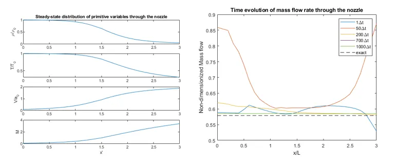
The above programs were run for 1400 iterations which is more than enough for the solution to reach the steady-state in both cases. At the end of the simulation, the variables were plotted along the nozzle and compared with the analytical solution from [1].
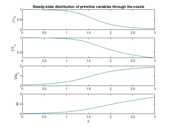
The above figure shows the distribution of the primitive variables along the nozzle at steady-state. These variables were obtained from the non-conservation equations. But how does these values reach the steady-state. A plot representing the evolution of the primitive variables with iteration is shown below:
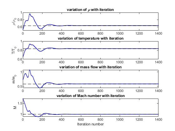
It can be observed that the maximum change takes place in the early time-steps and then it reaches the steady-state value asymptotically. There is a small difference between the numerical value and the exact value, even after convergence.
Another interesting aspect is to look at the evolution of mass flow rate with time.
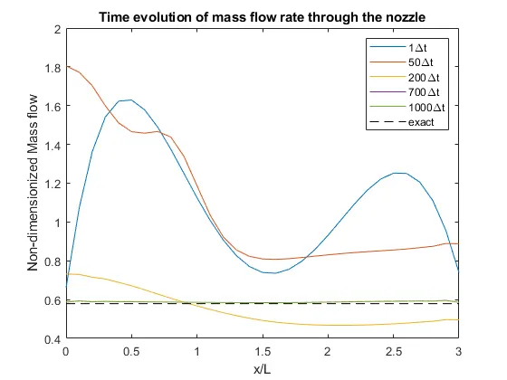
The above figure shows the variation of mass flow rate along the nozzle at different time-steps. It can be observed that at steady-state mass flow achieves a constant value which is equal to the steady-state value.
Similar results were obtained from the conservation equations as shown below:
Then what is the difference between the conservation and non-conservation forms of the equation. To understand this, the steady-state mass flow rate distribution obtained from the two equations are compared in the figure below. Note that the y-axis is zoomed in.
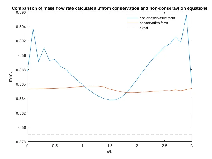
Essentially, the mass flow rate is constant through the nozzle with small variation of the order of `10^-3`. From the above figure, it can be observed that the steady-state mass flow distribution from the conservation form is more satisfactory than the non-conservation. The conservation form gives a distribution that is more closer to the analytical result. In contrast, the non-conservation result has a sizeable variation (in magnified scale) with some spurious oscillations at the inlet and the outlet.
This is because in the conservation form, the mass flow rate (`rho’*A’*V’`) is a primary variable which is solved during the iteration. On the other hand, in the non-conservation equation, the primitive variables are solved during iteration and the mass flow is obtained only as a secondary result. The conservation equation does a better job of preserving the mass flow rate.
Being an approximation, the numerical results are not equal to the analytical results. The finite difference approximation suffer majorly from the truncation error. In order to have a satisfactory result, this error needs to be reduced which can be achieved by reducing the value of `Deltax`. In other words increase the number of grid points in the domain. The above program was repeated with higher number of grid points to evaluate its influence on the final results. The following tables summarizes the values obtained from the simulation for comparison.
|
`(rho)/(rho_0)` |
`(T)/(T_0)` |
`(p)/(p_0)` |
M |
|
|
Exact solution |
0.634 |
0.833 |
0.528 |
1.000 |
|
Non-conservation form (31 points) |
0.639 |
0.837 |
0.534 |
0.999 |
|
Non-conservation form (61 points) |
0.638 |
0.835 |
0.533 |
0.999 |
|
conservation form (31 points) |
0.648 |
0.839 |
0.544 |
0.986 |
|
conservation form (61 points) |
0.638 |
0.835 |
0.533 |
0.999 |
From the above table the following conclusion can be obtained.
- The non-conservation equations provide a closer approximation of the primitive variables because they are the primary solution variables.
- By doubling the number of grid points, the numerical value move closer to the analytical solution.
- Increasing the number of grid points increases the computational time
- The conservation form of the equations required more computation time because of the extra step where the primitive variables are calculated from the primary variables.
References:
- McLay, A. "Computational Fluid Dynamics: the Basics with Applications, JD Anderson, McGraw-Hill Book Company Europe, McGraw-Hill House, Shoppenhangers Road, Maidenhead, Berkshire SL6 2QL. 1995. 547pp. Illustrated.£ 23.95." The Aeronautical Journal998 (1996): 365-365.
Appendix:
Plot function:
function [] = plot_variables(x,a,nt,rho_plot,v_plot,t_plot,p_plot,m_plot,M_plot)

    rho = rho_plot(:,end);
    t = t_plot(:,end);
    v = v_plot(:,end);
    M = M_plot(:,end);

    figure()
    subplot(4,1,1)
    plot(x,rho);
    ylabel("\rho/\rho_0");
    title("Steady-state distribution of primitive variables through the nozzle");
    subplot(4,1,2)
    plot(x,t);
    ylabel("T/T_0");
    subplot(4,1,3)
    plot(x,v);
    ylabel("V/a_0");
    subplot(4,1,4)
    plot(x,M);
    ylabel("M");
    xlabel("x'");

    % variation of m with x and t
    plot_time = [1,50,200,700,1000];
    m_analytical = 0.579.*ones(length(x));
    figure()
    for i =1:length(plot_time)
        plot(x,m_plot(:,plot_time(i)));
        hold on;
    end
    plot(x,m_analytical,'--k')
    ylabel("Non-dimensionized Mass flow")
    xlabel("x/L");
    legend("1\Deltat","50\Deltat","200\Deltat","700\Deltat","1000\Deltat","exact");
    title("Time evolution of mass flow rate through the nozzle")

    % variation of primitive variables at the throat with time
    throat_loc = find(a==1);
    time_series_x = linspace(1,nt,nt);
    rho_throat = 0.634.*ones(length(time_series_x));
    t_throat = 0.833.*ones(length(time_series_x));
    M_throat = ones(length(time_series_x));
    m_throat = 0.579.*ones(length(time_series_x));

    figure()
    subplot(4,1,1)
    for k=1:nt
        plot(k,rho_plot(throat_loc,k),'ob','MarkerSize',0.7);
        hold on;

    end

    plot(time_series_x,rho_throat,'--k')
    % xlabel("Iteration number")
    ylabel("\rho/\rho_0")
    title("variation of \rho with iteration");

    %figure()
    subplot(4,1,2)
    for k=1:nt
        plot(k,t_plot(throat_loc,k),'ob','MarkerSize',0.7);
        hold on;

    end

    plot(time_series_x,t_throat,'--k')
    % xlabel("Iteration number")
    ylabel("T/T_0")
    title("variation of temperature with iteration");

    % figure()
    subplot(4,1,3)
    for k=1:nt
        plot(k,m_plot(throat_loc,k),'ob','MarkerSize',0.7);
        hold on;

    end

    plot(time_series_x,m_throat,'--k')
    % xlabel("Iteration number")
    ylabel("m/m_0")
    title("variation of mass flow with iteration");

    % figure()
    subplot(4,1,4)
    for k=1:nt
        plot(k,M_plot(throat_loc,k),'ob','MarkerSize',0.7);
        hold on;

    end

    plot(time_series_x,M_throat,'--k')
    xlabel("Iteration number")
    ylabel("M")
    title("variation of Mach number with iteration");
end
% function end