Simulation of a 1D Super-sonic nozzle flow simulation using Macormack Method
Converging Diverging Nozzle
Ramjets, scramjets, and rockets all use nozzles to accelerate hot exhaust to produce thrust as described by Newton's third law of motion. The amount of thrust produced by the engine depends on the mass flow rate through the engine, the exit velocity of the flow, and the pressure at the exit of the engine. The value of these three flow variables are all determined by the nozzle design.
A nozzle is a relatively simple device, just a specially shaped tube through which hot gases flow. Ramjets and rockets typically use a fixed convergent section followed by a fixed divergent section for the design of the nozzle. This nozzle configuration is called a convergent-divergent (CD nozzle). In a CD nozzle, the hot exhaust leaves the combustion chamber and converges down to the minimum area, or throat, of the nozzle. The throat size is chosen to choke the flow and set the mass flow rate through the system. The flow in the throat is sonic which means the Mach number is equal to one in the throat. Downstream of the throat, the geometry diverges and the flow is isentropically expanded to a supersonic Mach number that depends on the area ratio of the exit to the throat. The expansion of a supersonic flow causes the static pressure and temperature to decrease from the throat to the exit, so the amount of the expansion also determines the exit pressure and temperature. The exit temperature determines the exit speed of sound, which determines the exit velocity. The exit velocity, pressure, and mass flow through the nozzle determine the amount of thrust produced by the nozzle.
Converging Diverging nozzle, showing approximate flow velocity (v), together with the effect on temperature (T) and pressure (p)
Subsonic Supersonic Isentropic Flow
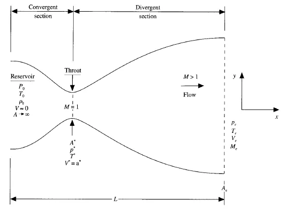
We consider the steady, isentropic flow through a convergent-divergent nozzle as per the above figure. The flow at the inlet to the nozzle comes from a reservoir where the pressure and temperature are denoted by `P_0` and `T_0` respectively. The cross-sectional area(`A`) of the reservoir is large ( `A to oo` ), and hence the velocity is very small ( `V to oo`). Thus, `P_0` and `T_0` are the stagnation values, or total pressure and total temperature, respectively. The flow expands sentrop1cally to supersonic speeds at the nozzle exit, where the exit pressure, temperature, velocity and Mach number are denoted by `P_e`, `T_e`, `V_e`, and `M_e`, respectively.
The area of the nozzle changes as a function of distance along with the x, and therefore in reality the flow field is two-dimensional (the flow varies in the two-dimensional `xy` space), we make the assumption that the flow properties-vary only with `x`. this is tantamount to assuming uniform flow properties across any given cross-section. Such flow is defined as quasi-one-dimensional flow.
The governing continuity, momentum, and energy equations for this quasi one-
dimensional, steady, isentropic flow can be expressed, respectively, as
Continuity Equation
`rho_1A_1V_1=rho_2A_2V_2`
Momentum Equation
`rho_1A_1+rho_1V_1^2A_1+int_(A_1)^(A_2)rho*dA=rho_2A_2+rho_2V_2^2A_2`
Energy Equation
`h_1+V_1^2/2=h_2+V_2^2/2`
where h=`h=c_pT`
The governing flow equations will be couched in terms of partial differential
equations suitable for the time-marching solution of quasi-one-dimensional flow
as the closed-form algebraic equations discussed above are not suitable for the present purpose.
To satisfy the overall physical principles of conservation of mass, newtons second law and energy conservation we apply the integral form of governing equations.
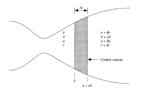
Continuity Equation (Integral Form)
`del/(delt)intintint_(spacial)rhodV+intint_(surface)rhoVdS=0`
`del/(delt)intintint_(spacial)rhodV=del/(delt)(rhoAdx)`
`intint_(surface)rhoVdS=-rhoVA+(rho+drho)(V+dV)(A+dA)`
As `dx` is very small, the terms involving products of differentials such as `p dV dA`, `dp dV dA`, go to zero much faster than those terms involving only one differential. Hence all terms involving products of differentials can be dropped, yielding in the limit as dx becomes very small.
`intint_(surface)rhoVdS=rhoVdA+rhoAdV+AVdrho=d(rhoAV)`
Substituing the values of `intint_(surface)rhoVdS` and `del/(delt)intintint_(spacial)rhodV` in the continuity equation we get a partial differential equation with respect to `x`.
`(del(rhoA))/(delt)+(del(rhoAV))/(delx)=0`
The partial differential equation form of the continuity equation suitable for unsteady, quasi-one-dimensional flow. It ensures that mass is conserved for this model of the flow.
Momentum Equation (Integral Form)
The integral form of the x component of the momentum
equation, for an inviscid flow (neglecting the viscous stress terms) with no body forces.
`del/(delt)intintint_(spacial)(rhou)dV+intint_(surface)(rhouV)dS=-intint_(surface)(PdS)_x`
where the term `(PdS)_x` denotes the `x` component of the vector `PdS`.
`del/(delt)intintint_(spacial)(rhou)dV=del/(delt)(rhoVAdx)`
`intint_(surface)(rhouV)dS=-rhoV_2A+(rho+drho)(V+dV)^2(A+dA)`
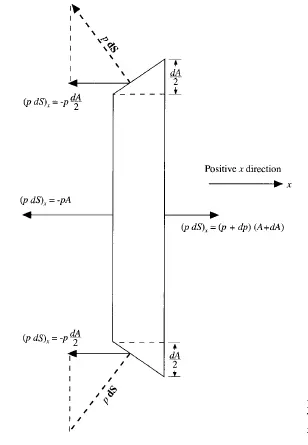
`intint_(surface)(PdS)_x=-PA+(P+dP)(A+dA)-2P((dA)/2)`
Substituing `del/(delt)intintint_(spacial)(rhou)dV`,`intint_(surface)(rhouV)dS` and `intint_(surface)(PdS)_x` the in momentum equation.
`(del(rhoVA))/(delt)+(del(rhoV^2A))/(delx)=-A(delP)/(delx)`
The above equation represents conservation form of the momentum equation for quasi-one-dimensional flow.
To obtain equivalent nonconservation form the above equation has multiplied the continuity equation by V.
`rho(dV)/(dt)+rhoV(delV)/(delx)=-(delP)/(delx)`
The below figure show forces in the x-direction acting on the control volume.
Energy Equation (Integral Form)
Consider the integral form of the energy equation for an adiabatic flow (`q = 0`) with nobody forces and no viscous effects, the integral form of the energy equation is
`del/(delt)intintint_(spacial)rho(e+V^2/2)dV+intint_(surface)rho(e+V^2/2)VdS=-intint_(surface)(PV)dS`
Applying the control volume to as per the shaded region and keeping in mind the pressure forces
`del/(delt)[rho(e+V^2/2)Adx]-rho(e+V^2/2)VA+(rho+deho)[e+de+((V+dV)^2)/2](V+dV)(A+dA)=-[-PVA+(P+dP)(V+dV)(A+dA)-2(PV(dA)/2)]`
Taking the limit as `dx` approaches zero, the above eqiation becomes the below partial differential equation
`(del[rho(e+V^2/2)A])/(delt)+(del[rho(e+V^2/2)VA])/(delx)=-(del(PAV))/(delx)`
The above equation is in the conservation form of the energy equation expressed in terms of the total energy `(e+V^2/2)`, appropriate for unsteady, quasi-one-dimensional flow.
Using the above equation non-conservation form of the energy equation in terms of internal energy can be found as
`rho(dele)/(delt)+rhoV(dele)/(delx)=-P(delV)/(delx)-PV(del(lnA))/(delx)`
The above equation for a calorically perfect gas can be directly used to form the energy equation in terms of temperature T.
`e=C_VT`
`rhoC_V(delT)/(delt)+rhoVC_V(delT)/(delx)=-P(delV)/(delx)-PV(del(lnA))/(delx)`
Discretising
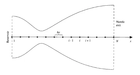
To implement a finite-difference solution, we divide the x-axis along with the nozzle into a number of discrete grid points. The points are evenly distributed along the x-axis, with `Deltax` denoting the spacing between grid points. The last point, namely, that at the nozzle exit, is denoted by `n`.
%Discretising
n=31;           %Number of Nodes
l=3;            %Length
dx=l/(n-1);     %dx=l/(n-1);
x=(0:dx:l);     %Discretised Domain
Calculation of Time Step
The governing system of equations is hyperbolic with respect to time.
`Deltat=C(Deltax)/(a+v)`
where `C` is the Courant Nuber and `a` is the speed of sound.
In the given problem, the flows changes form subsonic to supersonic and for stability, we need to have `C<=1`. The exact stability criterion for a linear equation `C<=1`, can only be viewed as general guidance for our present nonlinear problem as the speed varies.
Two approaches for finding the `Deltat`
Approach-1 Finding the local instantaneous `Deltat`
`(Deltat)_i^t=C(Deltax)/(a_i^t+V_i^t)`
This approach has a limitation as, such a local time-stepping approach does not realistically follow the actual, physical transients in the flow and hence cannot be used for an accurate solution of the unsteady flow.
Approach-2 Finding the global `Deltat`
The value of all local instantaneous `Deltat` are found at all grid points and the minimum value is used as `Deltat`.
This time marching solution is following the actual unsteady flow variations that would exist in nature. that is the solution gives a time-accurate solution of the actual transient flow field, consistent with the unsteady continuity, momentum and energy equations.
%Finding dt values as per CFL Criteria
for q=1:length(x)
    a=T.^0.5;
    C=0.5;
    dt(q)=(C*dx)/(a(q)+v(q));
end
dt=min(dt); %Choosing the minimum value
Boundary Conditions
Boundary conditions are important aspects because without the physically proper implementation of boundary conditions and they are proper numerical representation, the solution to the problem will not converge or else will give false results.
The gridpoint `1` and `n` represent the two boundary points on the x-axis. Point `1` is essentially in the reservoir and it represents the inflow boundary condition. The point `n` is an outflow boundary.
The area for the reservoir is theoretically infinite, and we are starting our own calculation at point l where the cross-sectional area is finite. Hence, the point is a subsonic inflow boundary and the speed at gridpoint 1 is not zero.
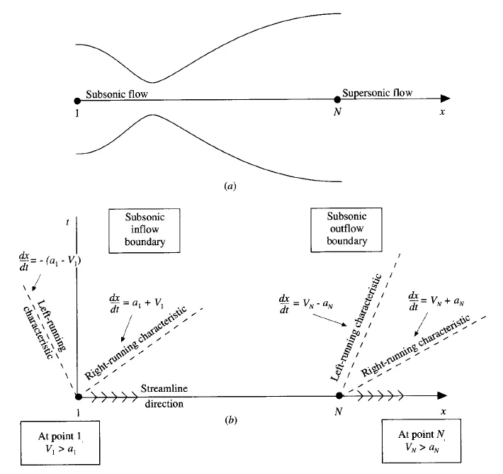
For the above unsteady inviscid flow is governed by hyperbolic equation and there exist two real characteristic lines through any point.
Consider Point 1
The local flow velocity V_1 is less than the speed of sound hence one characteristic curve traves towards the left and one characteristic towards the right. Therefore we can say that at the subsonic inflow boundary, we must stipulate the values of two dependent flow-field variables, whereas the value of one other variable must be allowed to float.
The method of characteristics tell us that at a boundary where one characteristic propagates into the domain, then the value of one dependent flow-field variable must be specified at that boundary, and if one characteristic line propagates out of the domain, then the
value of another dependent flow-field variable must be allowed to float at the boundary. That is it must be calculated in steps of time as a function of the timewise solution of the flow field.
The value of `V_1` changes with time and is calculated from information provided by the flow-field solution over the internal points.
`V_1=2V_2-V_3`
As point 1 is a reservoir the density and temperature are held fixed independent of time.
Consider Point n
At the supersonic outflow boundary, we have both characteristics propagating out of the domain. So does the streamline at point `n`.
Therefore, there are no flow-field variables that require their values to be stipulated at the supersonic outflow boundary, all variables must be allowed to float at this boundary.
At the point, `n` we must allow all the flow filed variables to float. We use extrapolation based on the flow field values at the internal points.
`V_n=2V_(n-1)-V_(n-2)`
`rho_n=2rho_(n-1)-rho_(n-2)`
`T_n=2T_(n-1)-T_(n-2)`
Applying Boundary Conditions
    %Apply the Boundary Conditions
    %Inlet
    v(1)=2*v(2)-v(3);

    %Outlet
    v(n)=2*v(n-1)-v(n-2);
    rho(n)=2*rho(n-1)-rho(n-2);
    T(n)=2*T(n-1)-T(n-2);
Non-Dimensionalise of Variables
The physical units are identified using the dimension of the variables, however, in computational fluid dynamics, the flow field variables are expressed in terms of nondimensional variables.
The non-dimensional variables `P/P_0`, `rho/rho_0` and `T/T_0` varies between 0 and 1
The reservoir temperature and density are denoted by `T_0`and `rho_0`, respectively, we define the nondimensional temperature and density respectively as `T'=T/T_0` and `rho'=rho/rho_0`.
The length L of the nozzle can be defined as the dimensionless length as`x'=x/L`.
The speed of the sound in the reservoir is `a_0` where `a_0=root()(gammaRT_0)`
The dimensionless velocity can be defined as `V'=V/a_0`
The quantity `L/a_0` has the dimension of the time and the dimensionless time can be defined as `t'=t/(L/a_0)`
The ratio of the local area `A` to the sonic throat area `A^ast` and the dimensionless area can be defined as `A'=A/A^ast`
Initial Conditions
`A=1+2.2(x-1.5)^2` where `x<=x<=3`
To start the time-marching calculations, we must stipulate initial conditions for `rho`, `T`, and `V` as a function of `x`, that is, we must set up values of `rho`, `T`, and `V` at time`t=0`.
`rho=1-0.3146x`
`T=1-0.2314x`
`V=(0.1+1.09x)T^(1/2)`
Applying Initial Conditions
%Calculate Initial Profiles
A=1+2.2*(x-1.5).^2;         %Area
rho=1-0.3146*x;             %Density
T=1-0.2314*x;               %Temperature
v=(0.1+1.09*x).*T.^0.5;     %Velocity
MacCormack method
The MacCormack technique is a two-step, predictor-corrector sequence that is used with the forward differencing on the predictor step and rearward differencing on the corrector step. It gives a second-order accurate method. MacCormack method does not require second-order derivatives hence making it simple compared to other solving techniques such as Lax-Wendroff Method.
Solving Non-Conservative Form using MacCormack Method
The initial values of flow variables are used to find the predicted values and the flow variables are computed for the entire domain and these values are referred to as predicted values.
Based on the predicted flow variables values the corrector steps derivatives are calculated and then the average of the predicted and the corrected derivative are used to find the final value of flow variables at each corresponding time step.
%Solution using Macormack Method

% Time Steps
nt=1400;

%Outer Time Loop
for k=1:nt

    rho_old=rho;
    v_old=v;
    T_old=T;

    %Predictor Method
    for j=2:n-1
        %drho_dt_p=-rho(j)*(v(j+1)-v(j))/dx-rho(j)*v(j)*(log(A(j+1))-log(A(j)))/dx-v(j)*(rho(j+1)-rho(j))/dx;
        dvdx=(v(j+1)-v(j))/dx;
        drhodx=(rho(j+1)-rho(j))/dx;
        dTdx=(T(j+1)-T(j))/dx;
        dlogAdx=(log(A(j+1))-log(A(j)))/dx;

        % Continuity Equation
        drho_dt_p(j)=-rho(j)*dvdx-rho(j)*v(j)*dlogAdx-v(j)*drhodx;

        % Momentum Equation
        dv_dt_p(j)=-v(j)*dvdx-(1/gama)*(dTdx+(T(j)/rho(j))*drhodx);

        % Energy Equation
        dT_dt_p(j)=-v(j)*dTdx-(gama-1)*T(j)*(dvdx+v(j)*dlogAdx);

        %Solution Update
        rho(j)=rho(j)+drho_dt_p(j)*dt;
        v(j)=v(j)+dv_dt_p(j)*dt;
        T(j)=T(j)+dT_dt_p(j)*dt;
    end

    %Corrector Method
    for j=2:n-1
        %drho_dt_p=-rho(j)*(v(j)-v(j-1))/dx-rho(j)*v(j)*(log(A(j))-log(A(j-1)))/dx-v(j)*(rho(j)-rho(j-1))/dx;
        dvdx=(v(j)-v(j-1))/dx;
        drhodx=(rho(j)-rho(j-1))/dx;
        dTdx=(T(j)-T(j-1))/dx;
        dlogAdx=(log(A(j))-log(A(j-1)))/dx;

        % Continuity Equation
        drho_dt_c(j)=-rho(j)*dvdx-rho(j)*v(j)*dlogAdx-v(j)*drhodx;

        % Momentum Equation
        dv_dt_c(j)=-v(j)*dvdx-(1/gama)*(dTdx+(T(j)/rho(j))*drhodx);

        % Energy Equation
        dT_dt_c(j)=-v(j)*dTdx-(gama-1)*T(j)*(dvdx+v(j)*dlogAdx);

    end

    %Computing the average time derivative
    drho_dt=0.5*(drho_dt_c+drho_dt_p);
    dv_dt=0.5*(dv_dt_c+dv_dt_p);
    dT_dt=0.5*(dT_dt_c+dT_dt_p);

    %Final Solution Update
    for i=2:(n-1)
        rho(i)=rho_old(i)+drho_dt(i)*dt;
        v(i)=v_old(i)+dv_dt(i)*dt;
        T(i)=T_old(i)+dT_dt(i)*dt;

    end

    %Apply the Boundary Conditions
    %Inlet
    v(1)=2*v(2)-v(3);

    %Outlet
    v(n)=2*v(n-1)-v(n-2);
    rho(n)=2*rho(n-1)-rho(n-2);
    T(n)=2*T(n-1)-T(n-2);

end
Results on Solving Non-Conservative Form of Quasi 1D Subsonic-Supersonic Nozzle
Steady State Profile
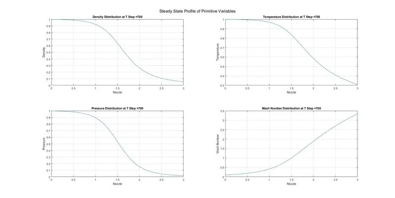
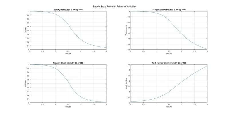
The steady-state profile of the primitive variables are shown below, we can see that when the flow becomes steady the density, pressure and temperature at the inlet is unity and the velocity at the inlet very less and as the flow approaches the nozzle throat the density, pressure and temperature decreases and the speed increases.
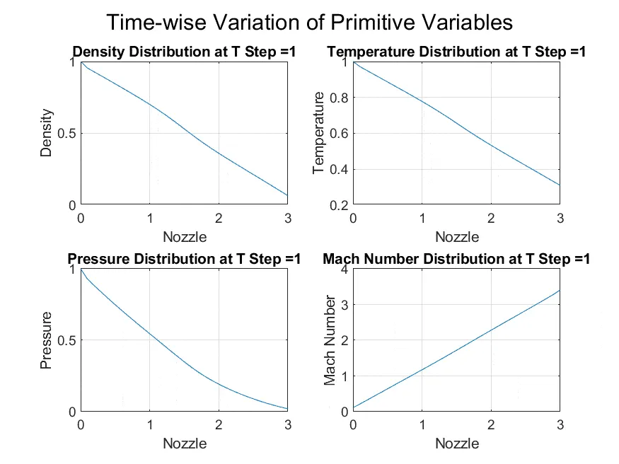
Flow Animation for 200 Timesteps
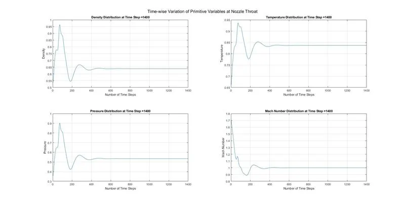
Time-wise Variation of Primitive Variables at Nozzle Throat
The variation at of the primitive of rho, T, P and Mach Number at nozzle throat is plotted versus time number of time steps. The abscissa starts at 0 and goes up to 1400. The large changes are seen at initial time steps and with the increase in time steps as it approaches steady state the changes becomes smaller and smaller and at about 700 times step it becomes stable.
Mass Flow Rate through the Nozzle at Different Time Steps
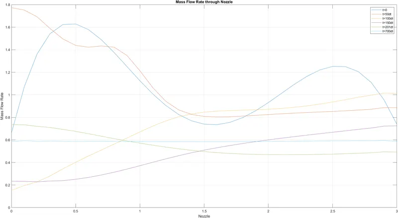
The mass flow rate curve for different time step is plotted to check the mass flow at different nodes of the nozzle at varying time steps. It is seen that the mass flow rate varies considerably up to 200-time steps and begins to settle down.
At 700-time steps, the mass flow distribution is a straight, horizontal line across the graph. This says that the mass flow has converged to a constant, steady-state value
throughout the nozzle.
`rhoVA=0.579`
Solving Conservative Form using MacCormack Method
Boundary Conditions
At Inflow
At the subsonic inflow boundary, two properties are held fixed and one is allowed to float, and at the supersonic outflow boundary, all properties are allowed to float.
`u_(1_(i=1))=(rhoA)_(i=1)=FixedValue`
`u_(2_(i=1))=2u_(2_(i=2))-u_(2_(i=3))`
`u_(3_(i=1))=u_(1_(i=1))(T_(i=1)/(gamma-1)+gamma/2V_(i=1)^2)`
At Outflow
At the point, `n` we must allow all the flow filed variables to float. We use extrapolation based on the flow field values at the internal points.
`(u_1)_n=2(u_1)_(n-1)-(u_1)_(n-2)`
`(u_2)_n=2(u_2)_(n-1)-(u_2)_(n-2)`
`(u_3)_n=2(u_3)_(n-1)-(u_3)_(n-2)`
Applying Boundary Conditions
%Apply the Boundary Conditions
    %Inlet
    u1(1)=rho(1)*A(1);
    u2(1)=2*u2(2)-u2(3);
    v(1)=u2(1)/u1(1);
    T(1)=(gama-1)*((u3(1)/u1(1))-(gama/2)*(u2(1)/u1(1))^2);
    u3(1)=u1(1)*((T(1))/(gama-1)+(gama/2)*(v(1)^2));

    %Outlet
    u1(n)=2*u1(n-1)-u1(n-2);
    u2(n)=2*u2(n-1)-u2(n-2);
    u3(n)=2*u3(n-1)-u3(n-2);
Initial Conditions
The dependent variables being solved are `u_1`, `u_2`, and `u_3`, we need initial conditions for these variables at time t = 0 in order to start the finite-difference solution.
`A=1+2.2(x-1.5)^2` where `x<=x<=3`
For `0<=x<=0.5`
`rho=1`
`T=1`
For `0.5<=x<=1.5`
`rho=1-0.366(x-0.5)`
`T=1-0.167(x-0.5)`
For `1.5<=x<=3.5`
`rho=0.634-0.3879(x-1.5)`
`T=0.833-0.3507(x-1.5)`
The conservative form of the equation is more sensitive to hence for stability we need to provide an improved initial condition for the solution to converge.
The velocity `V` is defined taking into considering the `u_2=rhoAV` and assuming a constant mass flow rate.
`V=u_2/(rhoA)=0.59/(rhoA)`
The value 0.59 is chosen for `u_2`because it is close to the exact analytical value of the steady-state mass flow (which for this case is 0.579).
Applying Initial Conditions
%Calculate Initial Condition
for ct=1:length(x)
   if(0<=x(ct) && x(ct)<=0.5)
       rho(ct)=1;
       T(ct)=1;
   end

   if(0.5<=x(ct) && x(ct)<=1.5)
       rho(ct)=1-0.366*(x(ct)-0.5);
       T(ct)=1-0.167*(x(ct)-0.5);
   end

   if(1.5<=x(ct) && x(ct)<=3.5)
       rho(ct)=0.634-0.3879*(x(ct)-1.5);
       T(ct)=0.833-0.3507*(x(ct)-1.5);
    end
end

%Calculate Initial Profiles
A=1+2.2*(x-1.5).^2;         %Area
p=rho.*T;                   %Pressure
u2=0.59.*ones(1,n);        %Solution Variable
v=u2./(rho.*A);             %Velocity
Implementing MacCormack Method for Conservative form of Equation
The governing equation for the conservative form of the equation is expressed in form of solution vector `u`, flux vector `f` and the source `j`. The elements of the solutions vector are defined using the non dimensionalised primitive values as
`u_1=rhoA`
`u_2=rhoAV`
`u_3=rho(e/(gamma-1)+gamma/2V^2)A`
`f_1=rhoAV`
`f_2=rhoAV^2+1/gammarhoA`
`f_3=rho(e/(gamma-1)+gamma/2V^2)VA+rhoAV`
`j_2=1/gammarho(delA)/(delx)`
The conservative form of the equation while solving using the primitive variables are show instabilities during the time marching solution which is assumed to cause by the lack of purity in the formulation.
This issue is solved by eliminating the primitive variables and finding the flux vector and source vector in terms of solution vector which avoids the computation of primitive variables at every time step.
`f_1=u_1`
`f_2=u_2^2/u_1+(gamma-1)/gamma(u_3-gamma/2(u_2^2/u_1))`
`f_3=gamma(u_2u_3)/u_1-(gamma(gamma-1))/2(u_2^3/u_1)`
`j_2=(gamma-1)/gamma(u_3-gamma/2u_2^2/u_1)(del(lnA))/(delx)`
Now we can proceed with solving the equation as we have found the solution vector, flux and the true source values using the initial values of flow variables. Now we fin the predicted values with forward differencing and update the values of the solution, flux and true source term. These updated values are used to find the corrector values using the backward differencing scheme. At each time step these steps for computed to find values at each node.
Based on the predicted and the corrector step derivatives we find the average derivative which is used to compute the final values of flow variables at each corresponding time step.
%Solution of Consrvative Form using Macormack Method

%Calculate Initial Condition
for ct=1:length(x)
   if(0<=x(ct) && x(ct)<=0.5)
       rho(ct)=1;
       T(ct)=1;
   end

   if(0.5<=x(ct) && x(ct)<=1.5)
       rho(ct)=1-0.366*(x(ct)-0.5);
       T(ct)=1-0.167*(x(ct)-0.5);
   end

   if(1.5<=x(ct) && x(ct)<=3.5)
       rho(ct)=0.634-0.3879*(x(ct)-1.5);
       T(ct)=0.833-0.3507*(x(ct)-1.5);
    end
end

%Calculate Initial Profiles
A=1+2.2*(x-1.5).^2;         %Area
p=rho.*T;                   %Pressure
u2=0.59.*ones(1,n);         %Solution Variable
v=u2./(rho.*A);             %Velocity


%Finding dt values as per CFL Criteria
for q=1:length(x)
    a=T.^0.5;
    C=0.5;
    dt(q)=(C*dx)/(a(q)+v(q));
end
dt=min(dt); %Choosing the minimum value


%Solution Vector
u1=rho.*A;
u2=rho.*A.*v;
u3=rho.*A.*((T./(gama-1))+gama*v.^2/2);

% Time Steps
ntc=700;

%Outer Time Loop
for k=1:ntc

    u1_old=u1;
    u2_old=u2;
    u3_old=u3;

    %Flux term
    f1=u2;
    f2=((u2.^2)./u1)+((gama-1)/gama)*(u3-(gama*u2.^2)./(2*u1));
    f3=((gama*u2.*u3)./u1)-((gama*(gama-1)/2)*((u2.^3)./(u1.^2)));

    rho=u1./A;
    T=(gama-1)*((u3./u1)-((gama/2)*(u2./u1).^2));

    %Source term
    for j=2:n-1
        %%Method 1
        %j2(j)=(1/gama)*rho(j)*T(j)*((A(j+1)-A(j))/(dx));
        %Method 2
        j2(j)=((gama-1)/gama)*(u3(j)-(gama/2)*(u2(j)^2/u1(j)))*((log(A(j+1))-log(A(j)))/(dx));
    end

    %Predictor Method
    for j=2:n-1

        %Continuity Equation
        du1_dt_p(j)=-(f1(j+1)-f1(j))/dx;

        %Momentum Equation
        du2_dt_p(j)=-((f2(j+1)-f2(j))/dx)+j2(j);

        %Energy Equation
        du3_dt_p(j)=-(f3(j+1)-f3(j))/dx;

        %Solution Update
        u1(j)=u1(j)+du1_dt_p(j)*dt;
        u2(j)=u2(j)+du2_dt_p(j)*dt;
        u3(j)=u3(j)+du3_dt_p(j)*dt;

    end

     %Apply the Boundary Conditions
    %Inlet
    u1(1)=rho(1)*A(1);
    u2(1)=2*u2(2)-u2(3);
    v(1)=u2(1)/u1(1);
    T(1)=(gama-1)*((u3(1)/u1(1))-(gama/2)*(u2(1)/u1(1))^2);
    u3(1)=u1(1)*((T(1))/(gama-1)+(gama/2)*(v(1)^2));

    %Outlet
    u1(n)=2*u1(n-1)-u1(n-2);
    u2(n)=2*u2(n-1)-u2(n-2);
    u3(n)=2*u3(n-1)-u3(n-2);

    %Corrector Method
        f1=u2;
        f2=((u2.^2)./u1)+((gama-1)/gama)*(u3-(gama*u2.^2)./(2*u1));
        f3=((gama*u2.*u3)./u1)-((gama*(gama-1)/2)*((u2.^3)./(u1.^2)));

        rho=u1./A;
        T=(gama-1)*((u3./u1)-((gama/2)*(u2./u1).^2));

    %Source term
    for j=2:n-1
        %%Method 1
        %j2(j)=(1/gama)*rho(j)*T(j)*((A(j)-A(j-1))/(dx));
        %Method 2
        j2(j)=((gama-1)/gama)*(u3(j)-(gama/2)*(u2(j)^2/u1(j)))*((log(A(j))-log(A(j-1)))/(dx));
    end


    for j=2:n-1

        % Continuity Equation
        du1_dt_c(j)=-(f1(j)-f1(j-1))/dx;

        % Momentum Equation
        du2_dt_c(j)=-((f2(j)-f2(j-1))/dx)+j2(j);

        % Energy Equation
        du3_dt_c(j)=-(f3(j)-f3(j-1))/dx;

    end

    %Compute the Average Time Derivative
    du1_dt=0.5*(du1_dt_c+du1_dt_p);
    du2_dt=0.5*(du2_dt_c+du2_dt_p);
    du3_dt=0.5*(du3_dt_c+du3_dt_p);

    %Final Solution Update
    for i=2:(n-1)
        u1(i)=u1_old(i)+du1_dt(i)*dt;
        u2(i)=u2_old(i)+du2_dt(i)*dt;
        u3(i)=u3_old(i)+du3_dt(i)*dt;

    end

    %Apply the Boundary Conditions
    %Inlet
    u1(1)=rho(1)*A(1);
    u2(1)=2*u2(2)-u2(3);
    v(1)=u2(1)/u1(1);
    T(1)=(gama-1)*((u3(1)/u1(1))-(gama/2)*(u2(1)/u1(1))^2);
    u3(1)=u1(1)*((T(1))/(gama-1)+(gama/2)*(v(1)^2));

    %Outlet
    u1(n)=2*u1(n-1)-u1(n-2);
    u2(n)=2*u2(n-1)-u2(n-2);
    u3(n)=2*u3(n-1)-u3(n-2);

    %Final Values
    rho=u1./A;                  %Density
    v=u2./(rho.*A);             %Velocity
    p=rho.*T;                   %Pressure
    %Temperature
    T=(gama-1)*((u3./u1)-(gama/2)*(u2./u1).^2);
    M=v./(T.^0.5);              %Mach Numer
    mdot=rho.*v.*A;             %Mass Flow rate


    %Storing Values with Time Step
    vcon(k,:)=v;                      %Velocity
    Tcon(k,:)=T;                      %Temperature
    rhocon(k,:)=rho;                  %Density
    pcon(k,:)=p;                      %Pressure
    Mcon(k,:)=M;                      %Mach Number
    mdotcon(k,:)=mdot;                %Mass Flow Rate
end
Results
In the conservation form, we assume the mass flow rate to be constant which makes is closer to the steady-state.
The steady-state profile using the conservative form of equation shows similar characteristics of primitive flow variables to non-conservative form.
Mass flow at different Time Step
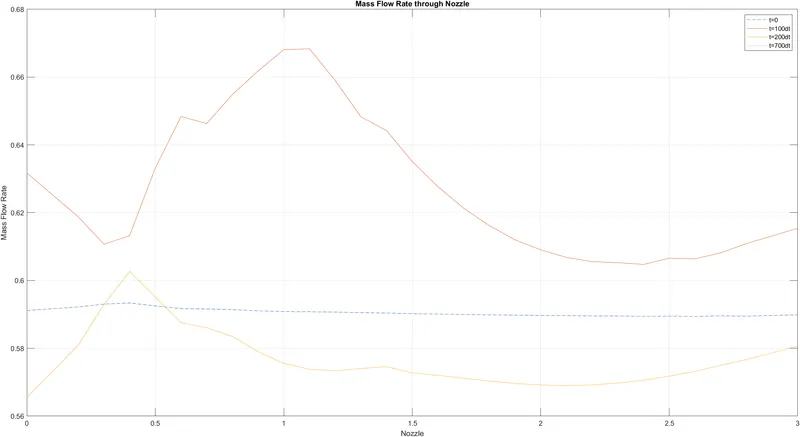
It is seen that the initial mass flow rate and the final result almost overlapping.
Inferences from the two methods
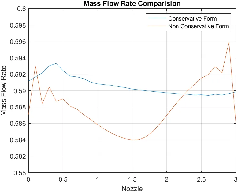
The advantage of the conservation form of the equations is that it does a better job of preserving mass throughout the flow field, mainly because the mass flow itself is one of the dependent variables in the equations the mass flow is a primary result from these equations.
In contrast, the non-conservation form of the equation takes dependent variables as the primitive flow variables and the mass flow rate is obtained as a secondary result.
Comparison of Mass flow for the two methods after 700-time steps.
Time taken for achieving steady-state is about 700-time steps which are in non dimensionalised form.
`t'=t/(L/a_0)`
`L/a_0=1/340.2=0.00294`
`t=(700*0.0204)*0.00294=0.042s`
The steady state is achived in 42 ms.
Grid Independence
To check for grid-independent we increase the increase or decrease the number of grid points. As in our case, we have taken the Courant number to be 0.5 which means we can increase our gridpoints up till the Courant number reaches 1. Increasing the number of gridpoints to double we doesnot see any major change in the results hence we can say that our solution is grid-independent.
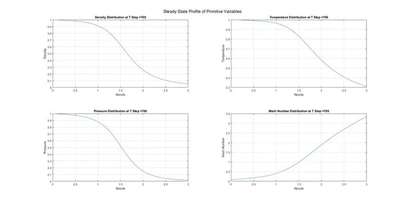
%Discretising
n=60;           %Number of Nodes
l=3;            %Length
dx=l/(n-1);     %dx=l/(n-1);
x=(0:dx:l);     %Discretised Domain

gama=1.4;       %Constant

%Solution of Non Consrvative Form using Macormack Method

%Calculate Initial Profiles
A=1+2.2*(x-1.5).^2;         %Area
rho=1-0.3146*x;             %Density
T=1-0.2314*x;               %Temperature
v=(0.1+1.09*x).*T.^0.5;     %Velocity

%Finding dt values as per CFL Criteria
for q=1:length(x)
    a=T.^0.5;
    C=0.5;
    dt(q)=(C*dx)/(a(q)+v(q));
end
dt=min(dt); %Choosing the minimum value

% Time Steps
ntn=700;

%Outer Time Loop
for k=1:ntn

    rho_old=rho;
    v_old=v;
    T_old=T;

    %Predictor Method
    for j=2:n-1
        %drho_dt_p=-rho(j)*(v(j+1)-v(j))/dx-rho(j)*v(j)*(log(A(j+1))-log(A(j)))/dx-v(j)*(rho(j+1)-rho(j))/dx;
        dvdx=(v(j+1)-v(j))/dx;
        drhodx=(rho(j+1)-rho(j))/dx;
        dTdx=(T(j+1)-T(j))/dx;
        dlogAdx=(log(A(j+1))-log(A(j)))/dx;

        % Continuity Equation
        drho_dt_p(j)=-rho(j)*dvdx-rho(j)*v(j)*dlogAdx-v(j)*drhodx;

        % Momentum Equation
        dv_dt_p(j)=-v(j)*dvdx-(1/gama)*(dTdx+(T(j)/rho(j))*drhodx);

        % Energy Equation
        dT_dt_p(j)=-v(j)*dTdx-(gama-1)*T(j)*(dvdx+v(j)*dlogAdx);

        %Solution Update
        rho(j)=rho(j)+drho_dt_p(j)*dt;
        v(j)=v(j)+dv_dt_p(j)*dt;
        T(j)=T(j)+dT_dt_p(j)*dt;
    end

    %Corrector Method
    for j=2:n-1
        %drho_dt_p=-rho(j)*(v(j)-v(j-1))/dx-rho(j)*v(j)*(log(A(j))-log(A(j-1)))/dx-v(j)*(rho(j)-rho(j-1))/dx;
        dvdx=(v(j)-v(j-1))/dx;
        drhodx=(rho(j)-rho(j-1))/dx;
        dTdx=(T(j)-T(j-1))/dx;
        dlogAdx=(log(A(j))-log(A(j-1)))/dx;

        % Continuity Equation
        drho_dt_c(j)=-rho(j)*dvdx-rho(j)*v(j)*dlogAdx-v(j)*drhodx;

        % Momentum Equation
        dv_dt_c(j)=-v(j)*dvdx-(1/gama)*(dTdx+(T(j)/rho(j))*drhodx);

        % Energy Equation
        dT_dt_c(j)=-v(j)*dTdx-(gama-1)*T(j)*(dvdx+v(j)*dlogAdx);

    end

    %Computing the average time derivative
    drho_dt=0.5*(drho_dt_c+drho_dt_p);
    dv_dt=0.5*(dv_dt_c+dv_dt_p);
    dT_dt=0.5*(dT_dt_c+dT_dt_p);

    %Final Solution Update
    for i=2:(n-1)
        rho(i)=rho_old(i)+drho_dt(i)*dt;
        v(i)=v_old(i)+dv_dt(i)*dt;
        T(i)=T_old(i)+dT_dt(i)*dt;

    end

    %Apply the Boundary Conditions
    %Inlet
    v(1)=2*v(2)-v(3);

    %Outlet
    v(n)=2*v(n-1)-v(n-2);           %Velocity
    rho(n)=2*rho(n-1)-rho(n-2);     %Density
    T(n)=2*T(n-1)-T(n-2);           %Temperature

    %Final Values
    p=rho.*T;                       %Pressure
    M=v./T.^0.5;                    %Mach Number
    mdot=rho.*v.*A;                 %Mass Flow Rate

    %Storing Values with Time Step
    vnon(k,:)=v;                      %Velocity
    Tnon(k,:)=T;                      %Temperature
    rhonon(k,:)=rho;                  %Density
    pnon(k,:)=p;                      %Pressure
    Mnon(k,:)=M;                      %Mach Number
    mdotnon(k,:)=mdot;                 %Mass Flow Rate

end

    %Steady State Distribution of Primitive Variables
    figure(4);
    subplot(2,2,1);
    plot(x,rho);
    title(sprintf('Density Distribution at T Step =%d',k));
    xlabel('Nozzle');
    ylabel('Density');
    grid on

    subplot(2,2,2);
    plot(x,T);
    title(sprintf('Temperature Distribution at T Step =%d',k));
    xlabel('Nozzle');
    ylabel('Temperature');
    grid on

    subplot(2,2,3);
    plot(x,p);
    title(sprintf('Pressure Distribution at T Step =%d',k));
    xlabel('Nozzle');
    ylabel('Pressure');
    grid on

    subplot(2,2,4);
    plot(x,M);
    title(sprintf('Mach Number Distribution at T Step =%d',k));
    xlabel('Nozzle');
    ylabel('Mach Number');
    grid on
    sgtitle('Steady State Profile of Primitive Variables');
Complete Program
clear all
close all
clc

%Discretising
n=31;           %Number of Nodes
l=3;            %Length
dx=l/(n-1);     %dx=l/(n-1);
x=(0:dx:l);     %Discretised Domain

gama=1.4;       %Constant

%Solution of Non Consrvative Form using Macormack Method

%Calculate Initial Profiles
A=1+2.2*(x-1.5).^2;         %Area
rho=1-0.3146*x;             %Density
T=1-0.2314*x;               %Temperature
v=(0.1+1.09*x).*T.^0.5;     %Velocity

%Finding dt values as per CFL Criteria
for q=1:length(x)
    a=T.^0.5;
    C=0.5;
    dt(q)=(C*dx)/(a(q)+v(q));
end
dt=min(dt); %Choosing the minimum value

% Time Steps
ntn=700;

%Outer Time Loop
for k=1:ntn

    rho_old=rho;
    v_old=v;
    T_old=T;

    %Predictor Method
    for j=2:n-1
        %drho_dt_p=-rho(j)*(v(j+1)-v(j))/dx-rho(j)*v(j)*(log(A(j+1))-log(A(j)))/dx-v(j)*(rho(j+1)-rho(j))/dx;
        dvdx=(v(j+1)-v(j))/dx;
        drhodx=(rho(j+1)-rho(j))/dx;
        dTdx=(T(j+1)-T(j))/dx;
        dlogAdx=(log(A(j+1))-log(A(j)))/dx;

        % Continuity Equation
        drho_dt_p(j)=-rho(j)*dvdx-rho(j)*v(j)*dlogAdx-v(j)*drhodx;

        % Momentum Equation
        dv_dt_p(j)=-v(j)*dvdx-(1/gama)*(dTdx+(T(j)/rho(j))*drhodx);

        % Energy Equation
        dT_dt_p(j)=-v(j)*dTdx-(gama-1)*T(j)*(dvdx+v(j)*dlogAdx);

        %Solution Update
        rho(j)=rho(j)+drho_dt_p(j)*dt;
        v(j)=v(j)+dv_dt_p(j)*dt;
        T(j)=T(j)+dT_dt_p(j)*dt;
    end

    %Corrector Method
    for j=2:n-1
        %drho_dt_p=-rho(j)*(v(j)-v(j-1))/dx-rho(j)*v(j)*(log(A(j))-log(A(j-1)))/dx-v(j)*(rho(j)-rho(j-1))/dx;
        dvdx=(v(j)-v(j-1))/dx;
        drhodx=(rho(j)-rho(j-1))/dx;
        dTdx=(T(j)-T(j-1))/dx;
        dlogAdx=(log(A(j))-log(A(j-1)))/dx;

        % Continuity Equation
        drho_dt_c(j)=-rho(j)*dvdx-rho(j)*v(j)*dlogAdx-v(j)*drhodx;

        % Momentum Equation
        dv_dt_c(j)=-v(j)*dvdx-(1/gama)*(dTdx+(T(j)/rho(j))*drhodx);

        % Energy Equation
        dT_dt_c(j)=-v(j)*dTdx-(gama-1)*T(j)*(dvdx+v(j)*dlogAdx);

    end

    %Computing the average time derivative
    drho_dt=0.5*(drho_dt_c+drho_dt_p);
    dv_dt=0.5*(dv_dt_c+dv_dt_p);
    dT_dt=0.5*(dT_dt_c+dT_dt_p);

    %Final Solution Update
    for i=2:(n-1)
        rho(i)=rho_old(i)+drho_dt(i)*dt;
        v(i)=v_old(i)+dv_dt(i)*dt;
        T(i)=T_old(i)+dT_dt(i)*dt;

    end

    %Apply the Boundary Conditions
    %Inlet
    v(1)=2*v(2)-v(3);

    %Outlet
    v(n)=2*v(n-1)-v(n-2);           %Velocity
    rho(n)=2*rho(n-1)-rho(n-2);     %Density
    T(n)=2*T(n-1)-T(n-2);           %Temperature

    %Final Values
    p=rho.*T;                       %Pressure
    M=v./T.^0.5;                    %Mach Number
    mdot=rho.*v.*A;                 %Mass Flow Rate

    %Storing Values with Time Step
    vnon(k,:)=v;                      %Velocity
    Tnon(k,:)=T;                      %Temperature
    rhonon(k,:)=rho;                  %Density
    pnon(k,:)=p;                      %Pressure
    Mnon(k,:)=M;                      %Mach Number
    mdotnon(k,:)=mdot;                 %Mass Flow Rate

%Time-wise Variation of Primitive Variables
    figure(1);
    subplot(2,2,1);
    plot(x,rho);
    title(sprintf('Density Distribution at T Step =%d',k));
    xlabel('Nozzle');
    ylabel('Density');
    grid on

    subplot(2,2,2);
    plot(x,T);
    title(sprintf('Temperature Distribution at T Step =%d',k));
    xlabel('Nozzle');
    ylabel('Temperature');
    grid on

    subplot(2,2,3);
    plot(x,p);
    title(sprintf('Pressure Distribution at T Step =%d',k));
    xlabel('Nozzle');
    ylabel('Pressure');
    grid on

    subplot(2,2,4);
    plot(x,M);
    title(sprintf('Mach Number Distribution at T Step =%d',k));
    xlabel('Nozzle');
    ylabel('Mach Number');
    grid on
    sgtitle('Time-wise Variation of Primitive Variables');
    saveas(gcf,['Time-wise Variation of Primitive Variables' num2str(k) '.png']);
end


    %Time-wise Variation of Primitive Variables at Nozzle Throat
    figure(2);
    subplot(2,2,1);
    plot((1:ntn),rhonon(:,16));
    title(sprintf('Density Distribution at Time Step =%d',k));
    xlabel('Number of Time Steps');
    ylabel('Density');
    grid on

    subplot(2,2,2);
    plot((1:ntn),Tnon(:,16));
    title(sprintf('Temperature Distribution at Time Step =%d',k));
    xlabel('Number of Time Steps');
    ylabel('Temperature');
    grid on

    subplot(2,2,3);
    plot((1:ntn),pnon(:,16));
    title(sprintf('Pressure Distribution at Time Step =%d',k));
    xlabel('Number of Time Steps');
    ylabel('Pressure');
    grid on

    subplot(2,2,4);
    plot((1:ntn),Mnon(:,16));
    title(sprintf('Mach Number Distribution at Time Step =%d',k));
    xlabel('Number of Time Steps');
    ylabel('Mach Number');
    grid on
    sgtitle('Time-wise Variation of Primitive Variables at Nozzle Throat');

    %Mass Flow Rate through Nozzle
    figure(3)
    plot(x,mdotf(1,:))
    hold on
    plot(x,mdotf(50,:))
    plot(x,mdotf(100,:))
    plot(x,mdotf(150,:))
    plot(x,mdotf(200,:))
    plot(x,mdotf(700,:))
    grid on
    xlabel('Nozzle');
    ylabel('Mass Flow Rate');
    title('Mass Flow Rate through Nozzle')
    legend('t=0','t=50dt','t=100dt','t=150dt','t=201dt','t=700dt');

    %Steady State Distribution of Primitive Variables
    figure(4);
    subplot(2,2,1);
    plot(x,rho);
    title(sprintf('Density Distribution at T Step =%d',k));
    xlabel('Nozzle');
    ylabel('Density');
    grid on

    subplot(2,2,2);
    plot(x,T);
    title(sprintf('Temperature Distribution at T Step =%d',k));
    xlabel('Nozzle');
    ylabel('Temperature');
    grid on

    subplot(2,2,3);
    plot(x,p);
    title(sprintf('Pressure Distribution at T Step =%d',k));
    xlabel('Nozzle');
    ylabel('Pressure');
    grid on

    subplot(2,2,4);
    plot(x,M);
    title(sprintf('Mach Number Distribution at T Step =%d',k));
    xlabel('Nozzle');
    ylabel('Mach Number');
    grid on
    sgtitle('Steady State Profile of Primitive Variables');


%Solution of Consrvative Form using Macormack Method

%Calculate Initial Condition
for ct=1:length(x)
   if(0<=x(ct) && x(ct)<=0.5)
       rho(ct)=1;
       T(ct)=1;
   end

   if(0.5<=x(ct) && x(ct)<=1.5)
       rho(ct)=1-0.366*(x(ct)-0.5);
       T(ct)=1-0.167*(x(ct)-0.5);
   end

   if(1.5<=x(ct) && x(ct)<=3.5)
       rho(ct)=0.634-0.3879*(x(ct)-1.5);
       T(ct)=0.833-0.3507*(x(ct)-1.5);
    end
end

%Calculate Initial Profiles
A=1+2.2*(x-1.5).^2;         %Area
p=rho.*T;                   %Pressure
u2=0.59.*ones(1,n);         %Solution Variable
v=u2./(rho.*A);             %Velocity
u2old=u2;

%Finding dt values as per CFL Criteria
for q=1:length(x)
    a=T.^0.5;
    C=0.5;
    dt(q)=(C*dx)/(a(q)+v(q));
end
dt=min(dt); %Choosing the minimum value


%Solution Vector
u1=rho.*A;
u2=rho.*A.*v;
u3=rho.*A.*((T./(gama-1))+gama*v.^2/2);

% Time Steps
ntc=700;

%Outer Time Loop
for k=1:ntc

    u1_old=u1;
    u2_old=u2;
    u3_old=u3;

    %Flux term
    f1=u2;
    f2=((u2.^2)./u1)+((gama-1)/gama)*(u3-(gama*u2.^2)./(2*u1));
    f3=((gama*u2.*u3)./u1)-((gama*(gama-1)/2)*((u2.^3)./(u1.^2)));

    rho=u1./A;
    T=(gama-1)*((u3./u1)-((gama/2)*(u2./u1).^2));

    %Source term
    for j=2:n-1
        %%Method 1
        %j2(j)=(1/gama)*rho(j)*T(j)*((A(j+1)-A(j))/(dx));
        %Method 2
        j2(j)=((gama-1)/gama)*(u3(j)-(gama/2)*(u2(j)^2/u1(j)))*((log(A(j+1))-log(A(j)))/(dx));
    end

    %Predictor Method
    for j=2:n-1

        %Continuity Equation
        du1_dt_p(j)=-(f1(j+1)-f1(j))/dx;

        %Momentum Equation
        du2_dt_p(j)=-((f2(j+1)-f2(j))/dx)+j2(j);

        %Energy Equation
        du3_dt_p(j)=-(f3(j+1)-f3(j))/dx;

        %Solution Update
        u1(j)=u1(j)+du1_dt_p(j)*dt;
        u2(j)=u2(j)+du2_dt_p(j)*dt;
        u3(j)=u3(j)+du3_dt_p(j)*dt;

    end

     %Apply the Boundary Conditions
    %Inlet
    u1(1)=rho(1)*A(1);
    u2(1)=2*u2(2)-u2(3);
    v(1)=u2(1)/u1(1);
    T(1)=(gama-1)*((u3(1)/u1(1))-(gama/2)*(u2(1)/u1(1))^2);
    u3(1)=u1(1)*((T(1))/(gama-1)+(gama/2)*(v(1)^2));

    %Outlet
    u1(n)=2*u1(n-1)-u1(n-2);
    u2(n)=2*u2(n-1)-u2(n-2);
    u3(n)=2*u3(n-1)-u3(n-2);

    %Corrector Method
        f1=u2;
        f2=((u2.^2)./u1)+((gama-1)/gama)*(u3-(gama*u2.^2)./(2*u1));
        f3=((gama*u2.*u3)./u1)-((gama*(gama-1)/2)*((u2.^3)./(u1.^2)));

        rho=u1./A;
        T=(gama-1)*((u3./u1)-((gama/2)*(u2./u1).^2));

    %Source term
    for j=2:n-1
        %%Method 1
        %j2(j)=(1/gama)*rho(j)*T(j)*((A(j)-A(j-1))/(dx));
        %Method 2
        j2(j)=((gama-1)/gama)*(u3(j)-(gama/2)*(u2(j)^2/u1(j)))*((log(A(j))-log(A(j-1)))/(dx));
    end


    for j=2:n-1

        % Continuity Equation
        du1_dt_c(j)=-(f1(j)-f1(j-1))/dx;

        % Momentum Equation
        du2_dt_c(j)=-((f2(j)-f2(j-1))/dx)+j2(j);

        % Energy Equation
        du3_dt_c(j)=-(f3(j)-f3(j-1))/dx;

    end

    %Compute the Average Time Derivative
    du1_dt=0.5*(du1_dt_c+du1_dt_p);
    du2_dt=0.5*(du2_dt_c+du2_dt_p);
    du3_dt=0.5*(du3_dt_c+du3_dt_p);

    %Final Solution Update
    for i=2:(n-1)
        u1(i)=u1_old(i)+du1_dt(i)*dt;
        u2(i)=u2_old(i)+du2_dt(i)*dt;
        u3(i)=u3_old(i)+du3_dt(i)*dt;

    end

    %Apply the Boundary Conditions
    %Inlet
    u1(1)=rho(1)*A(1);
    u2(1)=2*u2(2)-u2(3);
    v(1)=u2(1)/u1(1);
    T(1)=(gama-1)*((u3(1)/u1(1))-(gama/2)*(u2(1)/u1(1))^2);
    u3(1)=u1(1)*((T(1))/(gama-1)+(gama/2)*(v(1)^2));

    %Outlet
    u1(n)=2*u1(n-1)-u1(n-2);
    u2(n)=2*u2(n-1)-u2(n-2);
    u3(n)=2*u3(n-1)-u3(n-2);

    %Final Values
    rho=u1./A;                  %Density
    v=u2./(rho.*A);             %Velocity
    p=rho.*T;                   %Pressure
    %Temperature
    T=(gama-1)*((u3./u1)-(gama/2)*(u2./u1).^2);
    M=v./(T.^0.5);              %Mach Numer
    mdot=rho.*v.*A;             %Mass Flow rate


    %Storing Values with Time Step
    vcon(k,:)=v;                      %Velocity
    Tcon(k,:)=T;                      %Temperature
    rhocon(k,:)=rho;                  %Density
    pcon(k,:)=p;                      %Pressure
    Mcon(k,:)=M;                      %Mach Number
    mdotcon(k,:)=mdot;                %Mass Flow Rate
end


%Steady State Profile of Primitive Variables
figure();
subplot(2,2,1);
plot(x,rho);
title(sprintf('Density Distribution at T Step =%d',k));
xlabel('Nozzle');
ylabel('Density');
grid on

subplot(2,2,2);
plot(x,T);
title(sprintf('Temperature Distribution at T Step =%d',k));
xlabel('Nozzle');
ylabel('Temperature');
grid on

subplot(2,2,3);
plot(x,p);
title(sprintf('Pressure Distribution at T Step =%d',k));
xlabel('Nozzle');
ylabel('Pressure');
grid on

subplot(2,2,4);
plot(x,M);
title(sprintf('Mach Number Distribution at T Step =%d',k));
xlabel('Nozzle');
ylabel('Mach Number');
grid on
sgtitle('Steady State Profile of Primitive Variables');

figure()
plot(x,mdotcon(k,:));
hold on
plot(x,mdotnon(k,:));
xlabel('Nozzle');
ylabel('Mass Flow Rate');
title('Mass Flow Rate Comparision');
axis([0 3 0.58 0.6]);
grid on
legend('Conservative Form','Non Conservative Form')


%Mass Flow Rate through Nozzle
figure()
plot(x,u2_old,'--')
hold on
plot(x,mdotcon(100,:))
plot(x,mdotcon(200,:))
plot(x,mdotcon(700,:),':')
grid on
xlabel('Nozzle');
ylabel('Mass Flow Rate');
title('Mass Flow Rate through Nozzle')
legend('t=0','t=100dt','t=200dt','t=700dt');
hold off
References
1. Computational Fluid Dynamics the Basics with Application by John D. Anderson Jr.