Developing MATLAB code using MacCormack Method for Simulation of a 1D quassi Super-sonic nozzle flow
Objective-
- To write code to solve the 1D supersonic nozzle flow equations using the Macormack Method by implementing both the conservative and non-conservative forms of the governing equations.
- Perform grid dependence test.
- To figure out the minimum number of cycles for which the simulation should be run in order for convergence.
- To Compare the normalized mass flow rate between the conservative forms and non-conservative forms.
MacCormack Method
In Computational Fluid Dynamics (CFD), MacCormack method is discretization scheme for the numerical solution of partial differential equations (PDE). The MacCormack method is a simpler variation of the two-step Lax-Wendroff scheme. This discretization scheme is proceeded by two steps: the predictor step and the corrector step.
i. Predictor step: the PDE is solved using a forward difference scheme
ii. Corrector step: the PDE is solved using backward difference scheme
The final solution is the average predictor step and a corrector step. MacCormack method is an excellent time-marching numerical scheme because it does not introduce diffusive errors in the solution.
Convergent-Divergent Nozzle
In this project, steady, isentropic flow through a convergent-divergent nozzle will be simulation as shown in Figure 1. The flow at the reservoir is considered at total pressure, `p_0` and total temperature, `T_0`. The cross-sectional area of the reservoir is large `(A→∞)`, hence, the velocity at inlet is very small (`V→0`). The flow expands isentropically to supersonic speed at the exit, where pressure, temperature, velocity, and Mach number denotes with e">`e`. The flow is subsonic (`M<1`) in the convergent section, goes through the throat area where it is at sonic speed (`M=1`) and becomes supersonic (`M>1`) at divergent section.
FIGURE 1 Schematic for subsonic-supersonic isentropic nozzle flow
Although the cross-sectional area, A, changes as a function of distance along with the nozzle, we make the assumption that the flow properties vary only in x-direction and properties are uniform in the y-direction. The assumption defines the flow as a quasi-one-dimensional flow.
Solutions of subsonic-supersonic nozzle flow are shown in Figure 2 from the textbook.
FIGURE 2 Isentropic subsonic-supersonic solution of quasi-one-dimesional nozzle flow.
Governing Equations
Using the integral form of continuity, momentum, and energy equations for a control volume with an infinitesimal thickness of the slice, `dx`.
Many CFD solutions are carried out directly in terms of dimensional variables, as shown above, however, for nozzle flows, the flow-field variables are frequently expressed in terms of nondimensional variables.
`x'=x/L` `V'=V/a_0` `t'=t/(L/a_0)` `A'=A/A⋅`
where
`a0=sqrt(γ⋅R⋅T0)` is speed of sound
A∗=">A∗== sonic throat area
Rewritting the non-conservative governing equations in nondimensional form:
Initial Conditions and Boundary Condition for Nonconservative form
ρ=1-0.3146xT=1-0.2314xV=(0.1+1.09x)T12]-for t=0">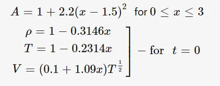
Using extrapolation, we get following boundary condition
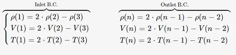
We can rewrite the generic form. Let's define the solution vector, U, the flux vector, F">F, and the source term, J">J as:
then the conservative equations become:
where;
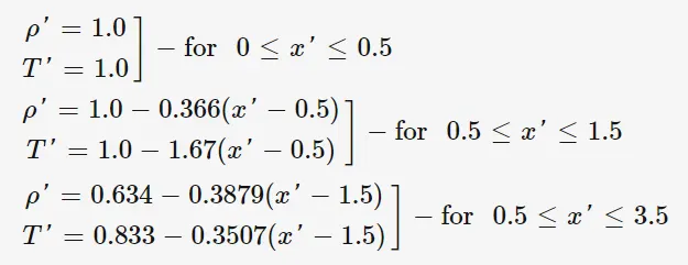
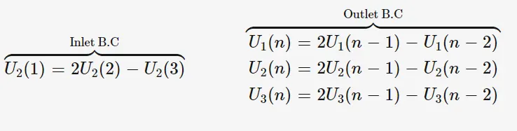
Initial conditions and Boundary conditions for conservative form
Initial Conditions:
Boundary Conditions:
Results
The profile of flow variables for Non-onservative form and Conservative form.
Variation of mass flow rate at different time steps.
Convergence-
Through the above two graphs the covergence time step can be analysed.We can see that at 700 time step the mass flow rate corresponds to the analytical solution which means steady state is achieved.
The convergence for non-onservative form and conservative form were found to be 404 and 471 iterations when the convergence criteria was used 1e-4.So we can conclude that the non-conservative form has faster convergence than the conservative form.
Comparision of mass flow rate between non-conservative form and conservative form.
From the above graph it can be concluded that mass flow rate in conservative form showed better results and corresponded to the analytical solution.
Simulation time for conservative and non conservative form
We can see from the results that Non-consevative form is faster than conservative form.
Grid Dependence test
Non conservative form(31 grids)
Conservative form (31 grids)
Non conservative form (61 grids)
Conservative form(61 grids)
From grid dependence test it can be seen that for 31 and 61 grid points respectively there was hardly any change in density,velocity,temperature and Mach number at the throat.This is noticed for both non conservative as well as conservative.So solution has no change for any number of grids.
Matlab Code:
Main program
close all;
clear all;
clc;
n=31;
x=linspace(0,3,n);
tol=1e-4;
m_analytical=0.579*ones(1,n);
[m_nc]=supersonic_nozzle_non_conservative(n,tol);
[m_c]=supersonic_nozzl_conservative(n,tol);
    figure(5)
    plot(x,m_nc,'linewidth',2)
    hold on
    plot(x,m_c,'linewidth',2)
    hold on
     plot(x,m_analytical,'linewidth',2)
    title('mass flow rate vs x')
    xlabel('x')
    ylabel('Mass flow rate')
    legend('Non-conservative','conservative','analytical')
function for Non-conservative form
function [m_nc]=supersonic_nozzle_non_conservative(n,tol)
tic
%grid
x=linspace(0,3,n);

dx=x(2)-x(1);
gamma=1.4;
%specify throat
throat=(n+1)/2;
 m_analytical=0.579*ones(1,n);

C=0.5;
%initial profiles
rho=1-0.3146*x;
t=1-0.2314*x;   %Temperature
v=(0.1+1.09*x).*t.^0.5;
rho_old=rho;
v_old=v;
t_old=t;
%area
a=1+2.2*(x-1.5).^2;
%time steps
nt=1400;
nt_step=linspace(1,nt,nt);
for p=1:n
    dt_a(p)=C*dx/(t(p)^0.5+v(p));
end
dt=min(dt_a);
%outer time loop
iter=1;
error_rho=9e9;
error_v=9e9;
error_t=9e9;
for k=1:nt
     rho_old=rho;
     v_old=v;
     t_old=t;


    %predictor method
    for j=2:n-1
        dvdx=(v(j+1)-v(j))/dx;
        drhodx=(rho(j+1)-rho(j))/dx;
        dtdx=(t(j+1)-t(j))/dx;
        dlogadx=(log(a(j+1))-log(a(j)))/dx;

        %continuity equation
        drhodt_p(j)=-rho(j)*dvdx-rho(j)*v(j)*dlogadx-v(j)*drhodx;

        %momentum equation
        dvdt_p(j)=-v(j)*dvdx-(1/gamma)*(dtdx+(t(j)/rho(j))*drhodx);

        %energy equation
        dtdt_p(j)=-v(j)*dtdx-(gamma-1)*t(j)*(dvdx+v(j)*dlogadx);

        %solution update
        rho(j)=rho(j)+drhodt_p(j)*dt;
        v(j)=v(j)+dvdt_p(j)*dt;
        t(j)=t(j)+dtdt_p(j)*dt;
    end
    %corrector method
    for j=2:n-1
        dvdx=(v(j)-v(j-1))/dx;
        drhodx=(rho(j)-rho(j-1))/dx;
        dtdx=(t(j)-t(j-1))/dx;
        dlogadx=(log(a(j))-log(a(j-1)))/dx;

        %continuity equation
        drhodt_c(j)=-rho(j)*dvdx-rho(j)*v(j)*dlogadx-v(j)*drhodx;

        %momentum equation
        dvdt_c(j)=-v(j)*dvdx-(1/gamma)*(dtdx+(t(j)/rho(j))*drhodx);

        %energy equation
        dtdt_c(j)=-v(j)*dtdx-(gamma-1)*t(j)*(dvdx+v(j)*dlogadx);

    end
 %compute avg time derivative
 drhodt=0.5*(drhodt_p+drhodt_c);
 dvdt=0.5*(dvdt_p+dvdt_c);
 dtdt=0.5*(dtdt_p+dtdt_c);

 %final solution update
 for i=2:n-1
 rho(i)=rho_old(i)+drhodt(i)*dt;
 v(i)=v_old(i)+dvdt(i)*dt;
 t(i)=t_old(i)+dtdt(i)*dt;
 end
 M=v./t.^0.5;
 m_nc=rho.*a.*v;
  m_nct(k,:)=rho.*a.*v;
   error_rho=max(abs(rho-rho_old));
  error_v=max(abs(v-v_old));
  error_t=max(abs(t-t_old));
  if (error_rho>tol && error_v>tol && error_t>tol)
      iter=iter+1;

  end
 %apply boundary conditions
 %inlet
 v(1)=2*v(2)-v(3);
 %outlet
  v(n)=2*v(n-1)-v(n-2);
   rho(n)=2*rho(n-1)-rho(n-2);
    t(n)=2*t(n-1)-t(n-2);


end
rho_throat=rho(throat);
  v_throat=v(throat);
   t_throat=t(throat);
    M_throat=M(throat);
 figure(1)
    subplot(4,1,2)
    plot(x,rho,'linewidth',2)

    xlabel('nozzle length')
    ylabel('density ratio')
    subplot(4,1,3)
    plot(x,v,'r','linewidth',2)

    xlabel('nozzle length')
    ylabel('velocity ratio')
    subplot(4,1,4)
    plot(x,t,'g','linewidth',2)

    xlabel('nozzle length')
    ylabel('Temperature ratio')
    subplot(4,1,1)
    plot(x,M,'m','linewidth',2)
    title(sprintf('No of timestep=%d, no of iteration to steady state=%d',k,iter))
    xlabel('nozzle length')
    ylabel('Mach number')
    suptitle('Non-conservative form')


     figure(3)
     plot(x,m_nct(50,:),x,m_nct(100,:),x,m_nct(200,:),x,m_nct(300,:),x,m_nct(500,:),'o',x,m_analytical,'linewidth',2)
     xlabel('non-dimensional distance x')
     ylabel('non-dimentional mass flow rate')
     title('variation of mass flow rate(non-conservative)')
     legend('50dt','100dt','200dt','300dt','700dt','analytical')
    time_nc=toc;
    fprintf('time of simlulation for nonconservative=%gsn',time_nc);
end
function for conservative form
function [m_c]=supersonic_nozzl_conservative(n,tol)
tic
%grid
x=linspace(0,3,n);
dx=x(2)-x(1);
gamma=1.4;
throat=(n+1)/2;
m_analytical=0.579*ones(1,n);
%initial profiles
for q=1:n
    if ((x(q)>=0) && (x(q)<=0.5))
    rho(q)=1;
    t(q)=1;
    elseif ((x(q)<1.5) && (x(q)>0.5))
        rho(q)=1-0.366*(x(q)-0.5);
        t(q)=1-0.167*(x(q)-0.5);
    elseif ((x(q)>=1.5) && (x(q)<=3.5))
        rho(q)=0.634-0.3879*(x(q)-1.5);
        t(q)=0.833-0.03507*(x(q)-1.5);
    end
end
%area
a=1+2.2*(x-1.5).^2;
 v=0.59./(rho.*a);
U1=rho.*a;
U2=rho.*a.*v;
U3=rho.*(t./(gamma-1)+(gamma/2)*v.^2).*a;
%time steps
nt=1400;
nt_step=linspace(1,nt,nt);
C=0.5;
for p=1:n
    dt_a(p)=C*dx/(t(p)^0.5+v(p));
end
    dt=min(dt_a);
%outer time loop
iter=1;
 error_rho=9e9;
 error_v=9e9;
 error_t=9e9;
for k=1:nt
     U1_old=U1;
     U2_old=U2;
     U3_old=U3;
     rho_old=U1_old./a;
    v_old=U2_old./U1_old;
    t_old=(gamma-1)*((U3_old./U1_old)-(gamma/2)*v_old.^2);
      F1=U2;
     F2=(U2.^2)./U1+((gamma-1)/gamma)*(U3-(gamma/2)*(U2.^2)./U1);
     F3=(gamma*U2.*U3)./U1-((gamma*(gamma-1)/2)*(U2.^3)./U1.^2);


    %predictor method
    for j=2:n-1
       J2(j)=(1/gamma)*rho(j)*t(j)*(a(j+1)-a(j))/dx;

        %continuity equation
        dU1dt_p(j)=-(F1(j+1)-F1(j))/dx;

        %momentum equation
        dU2dt_p(j)=J2(j)-(F2(j+1)-F2(j))/dx;

        %energy equation
        dU3dt_p(j)=-(F3(j+1)-F3(j))/dx;


        %solution update
        U1(j)=U1(j)+dU1dt_p(j)*dt;
        U2(j)=U2(j)+dU2dt_p(j)*dt;
        U3(j)=U3(j)+dU3dt_p(j)*dt;
    end
    rho=U1./a;
    v=U2./U1;
    t=(gamma-1)*((U3./U1)-(gamma/2)*v.^2);
    F1=U2;
     F2=(U2.^2)./U1+((gamma-1)/gamma)*(U3-(gamma/2)*(U2.^2)./U1);
     F3=(gamma*U2.*U3)./U1-((gamma*(gamma-1)/2)*((U2.^3)./(U1.^2)));

    %corrector method
    for j=2:n-1
         J2(j)=(1/gamma)*rho(j)*t(j)*(a(j)-a(j-1))/dx;
         %continuity equation
        dU1dt_c(j)=-(F1(j)-F1(j-1))/dx;

        %momentum equation
        dU2dt_c(j)=J2(j)-(F2(j)-F2(j-1))/dx;

        %energy equation
        dU3dt_c(j)=-(F3(j)-F3(j-1))/dx;


    end
 %compute avg time derivative
 dU1dt=0.5*(dU1dt_p+dU1dt_c);
 dU2dt=0.5*(dU2dt_p+dU2dt_c);
 dU3dt=0.5*(dU3dt_p+dU3dt_c);

 %final solution update
 for i=2:n-1
 U1(i)=U1_old(i)+dU1dt(i)*dt;
 U2(i)=U2_old(i)+dU2dt(i)*dt;
 U3(i)=U3_old(i)+dU3dt(i)*dt;
 end

 %apply boundary conditions
 %inlet

U1(1)=rho(1).*a(1);
  U2(1)=2*U2(2)-U2(3);
   v(1)=U2(1)/(rho(1)*a(1));
U3(1)=U1(1)*(t(1)/(gamma-1)+(gamma/2)*v(1)^2);
 %outlet
  U2(n)=2*U2(n-1)-U2(n-2);
   U1(n)=2*U1(n-1)-U1(n-2);
    U3(n)=2*U3(n-1)-U3(n-2);
    %updating vlues
    rho=U1./a;
    v=U2./U1;
    t=(gamma-1)*((U3./U1)-(gamma/2)*v.^2);
    M=v./t.^0.5;
 m_c=rho.*a.*v;
 m_nc(k,:)=rho.*a.*v;

    error_rho=max(abs(rho-rho_old));
    error_v=max(abs(v-v_old));
 error_t=max(abs(t-t_old));
  if (error_rho>tol && error_v>tol && error_t>tol)
      iter=iter+1;
  end

end
rho_throat=rho(throat);
  v_throat=v(throat);
   t_throat=t(throat);
    M_throat=M(throat);
 figure(2)
   subplot(4,1,2)
    plot(x,rho,'linewidth',2)

    xlabel('nozzle length')
    ylabel('density ratio')
    subplot(4,1,3)
    plot(x,v,'r','linewidth',2)

    xlabel('nozzle length')
    ylabel('velocity ratio')
    subplot(4,1,4)
    plot(x,t,'g','linewidth',2)

    xlabel('nozzle length')
    ylabel('Temperature ratio')
    subplot(4,1,1)
    plot(x,M,'m','linewidth',2)
    title(sprintf('No of timestep=%d ,no of iteration to steady state=%d',k,iter))
    xlabel('nozzle length')
    ylabel('Mach number')
    suptitle('Conservative form')


     figure(4)
     plot(x,m_nc(50,:),x,m_nc(100,:),x,m_nc(200,:),x,m_nc(300,:),x,m_nc(700,:),'o',x,m_analytical,'linewidth',2)
     xlabel('non-dimensional distance x')
     ylabel('non-dimentional mass flow rate')
     title('variation of mass flow rate(conservative)')
     legend('50dt','100dt','200dt','300dt','700dt','analytical')
      time_c=toc;
      fprintf('time of simlulation for conservative=%gsn',time_c);
end
Conclusion
1. For the conservation of mass, conservative form yields a better mass flow distribution compared to non-conservative form.
2. While comparing the solution from two forms of the equation, there is no clear answer to which one is better. However, non-conservative form yields slightly better results for the flow-field variables.
3. As we increase the number of grid points, the accuracy of the solution increases as well at the cost of computational time. Even though it is clear that that conservative form is faster, however, it is much harder to code compared to non-conservative form. This is because we have to break down the flow-field variable into flux variables, which is not needed in the non-conservative form.