Week 7: Shock tube simulation project
Aim:
- Setup a transient simulation through the shock tube.
- plot the cell count, pressure, and temperature plots wrt time.
Theory:
The shock tube is an instrument used to replicate and direct blast waves at a sensor or a model in order to simulate actual explosions and their effects, usually on a smaller scale. These are basically ducted into two different regions, one is a high-pressure region and another one is a low-pressure region, and these 2 ducts are closed on both sides. The diaphragm is placed between these two regions.
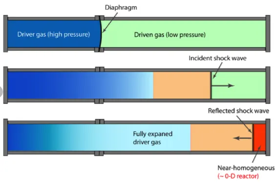
A shock wave inside a shock tube can be generated by a small explosion (blast-driven) or by the buildup of high pressures which cause diaphragm(s) to burst and a shock wave to propagate down the shock tube. Then the waves get reflected back and forth against the duct walls and this results in further mixing of the 2 species.
Shock tubes can also be used to study aerodynamic flow under a wide range of temperatures and pressures that are difficult to obtain in other types of testing facilities. These are also used to investigate compressible flow phenomena and gas-phase combustion reactions. More recently, shock tubes have been used in biomedical research to study how biological specimens are affected by blast waves.
Procedure:
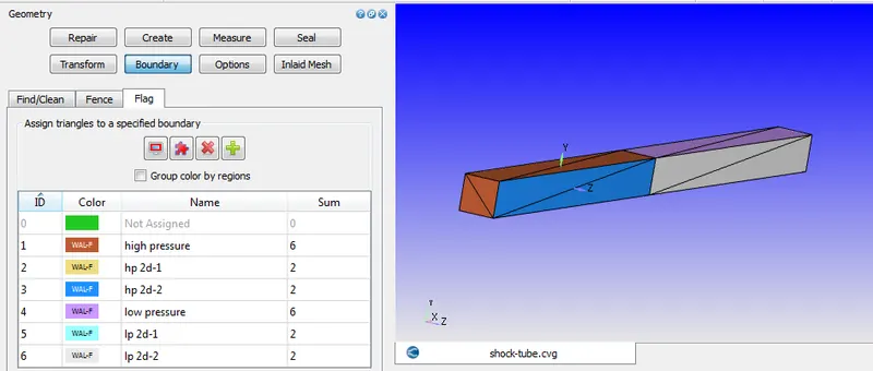
1. Geometry: Import the geometry and set the boundaries as a high-pressure body and low-pressure body. After applying the boundaries to the geometry check the normals pointed towards the flow.
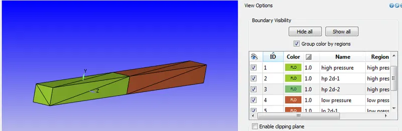
After the case setup, click on the view options > group colour by region. The green region belongs to high-pressure and the brown region belongs to low-pressure.
2. Case setup: Set application type to time-based.
2.1 Materials: Set as default variables.
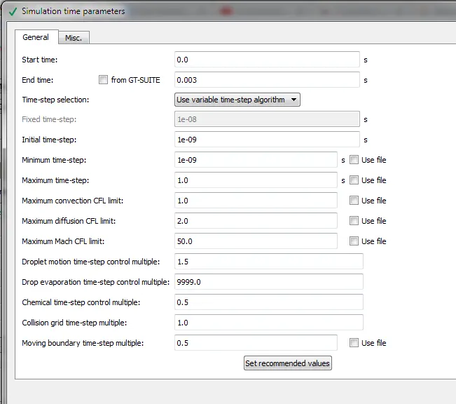
2.2 Simulation parameters: Set transient solver in the run parameters and set solver parameters to default.
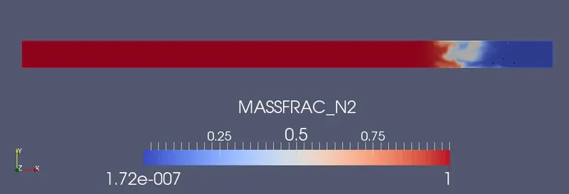
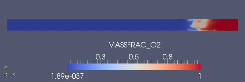
2.3 Initial conditions and events: Here there are 2 regions name as high and low regions. In the high-pressure region mention N2 as species and increase the pressure compared with the low-pressure region. In the low-pressure set O2 as species.
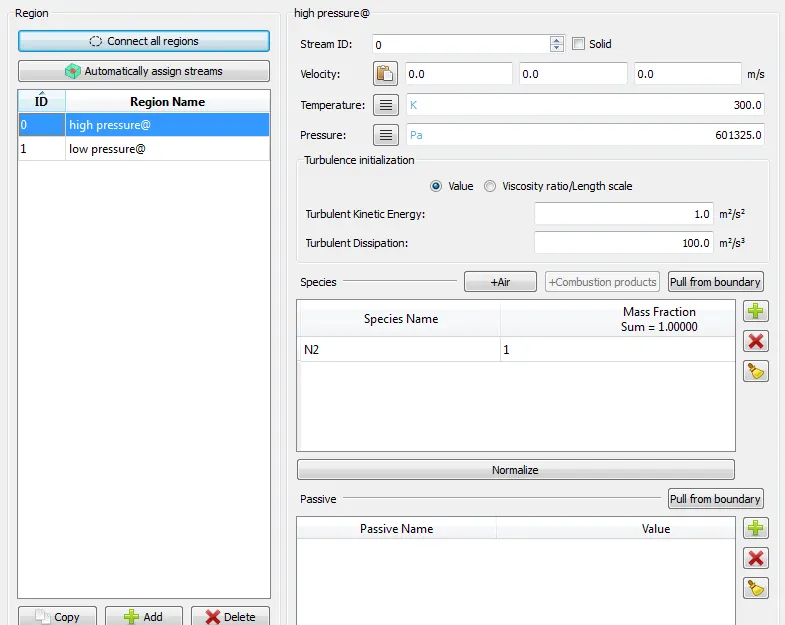
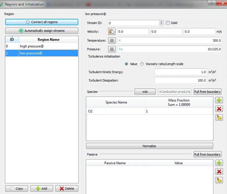
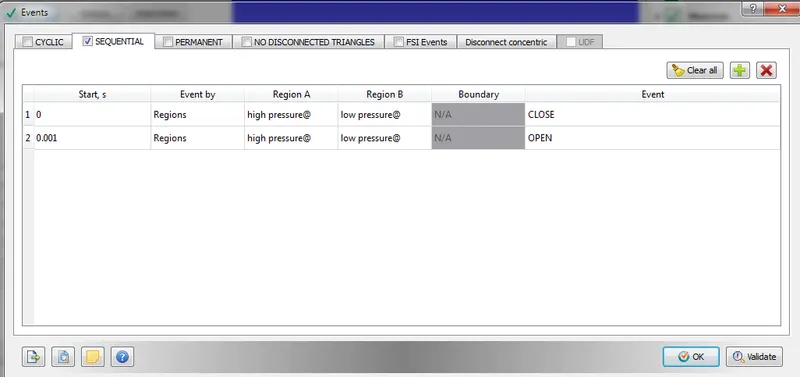
Open the events. The events are used when the 2 regions are in contact with each other with no boundary in between them. The events flag creates triangles in the place between the 2 regions called disconnect triangles. The events flag can be turned on before the case setup, by navigating to the initial conditions. After that, the event can be set by selecting the events(cyclic, sequential, and permanent) option in the case setup free. Here at 0 sec, the diaphragm closes and after 0.001 sec the diaphragm will open.
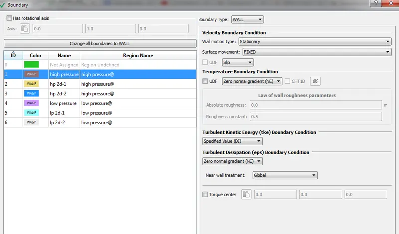
2.4 Boundaries: Here there is no inlet and outlet. So, for all boundary conditions set boundary type to wall and velocity boundary conditions to slip.
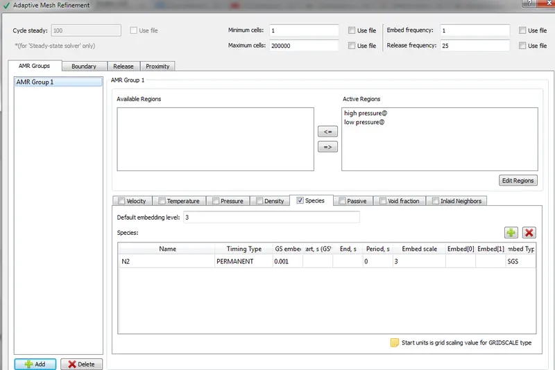
2.5 Grid control: Set mesh grid size to 0.002m and open adaptive mesh refinement.
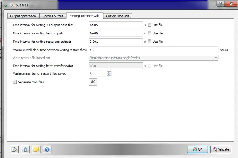
2.6 Output/post-processing:
3. Now export all input files: Click on files > Export > Export input files > choose the path and select all files and press ok.
4. Run the simulation and post-convert the files: Copy and paste the mpiexec.exe file and converge.exe file to the folder in which the input files are exported to run the simulation in Cygwin. Copy the post_convert_30_msmpi_64.exe file and paste it into the output folder. Now open Cygwin and go to the output folder and type mpiexec.exe -n 4 post_convert_30_msmpi_64.exe > enter the case name(as case1) > select file type as Paraview VTK in-line binary format > type all for files and cell variables and click enter (or) we can convert those files in converge studio.
5. Post-processing the files:
To post-process the files lanch paraview and open the file location as case1 which is saved in output > case1 .. vtm (this is a group file which is formed during post-converting the files) > click on apply > create a slice along the z-axis.
Results:
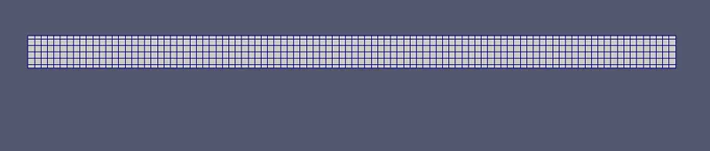
Mesh at 0-time step:-
Mesh at final time step:-

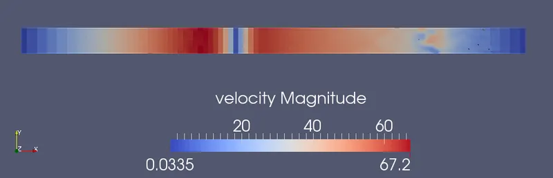
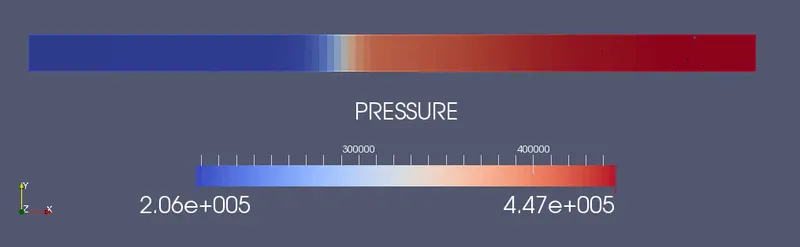
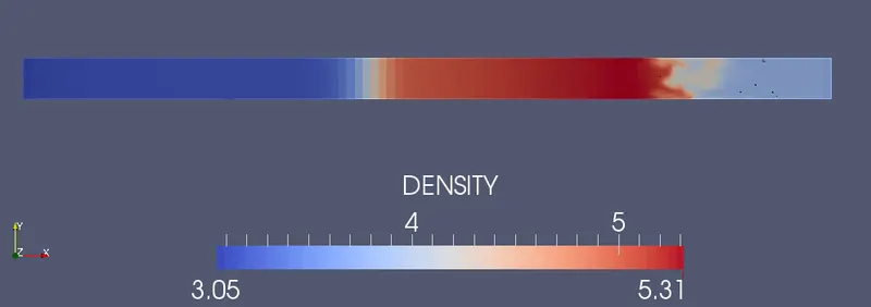
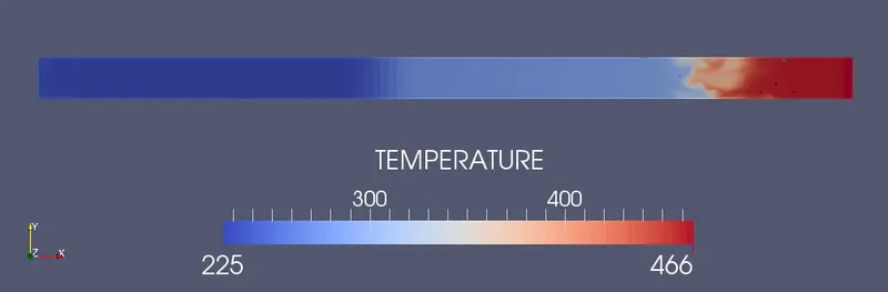
Contours for final time step:-
Plots:
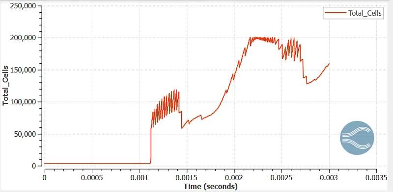
Total cells:
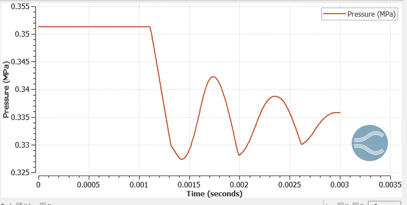
Average Pressure:
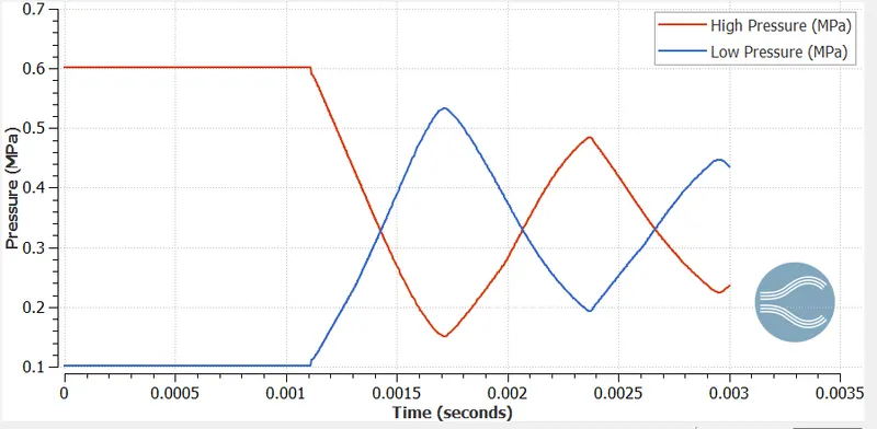
Pressure plot for high-pressure and low-pressure regions:
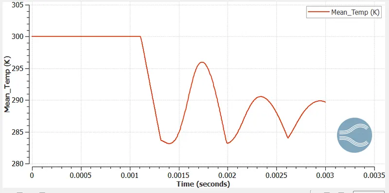
Mean temperature:
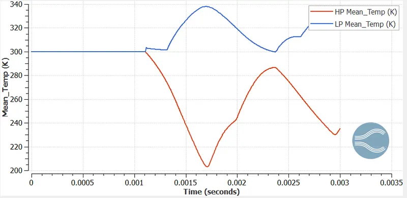
Mean temperature plot for high-pressure and low-pressure regions:
Animation links:
Conclusion:
- In the pressure plot, as the diaphragm is removed so the 2 regions are mixing with each other. So, the pressure in the high-pressure region drops from 6 bar to 1.4 bar in just a millisecond and then it keeps fluctuating. Similarly, the low-pressure region increases the pressure from 1 bar to 5.2 bar in a millisecond and then it keeps fluctuating.
- From the mean temperature for HP and LP regions plot, the high-pressure mean temperature suddenly drops from 300k to 200k within a millisecond, this sudden fluctuation is due to the shock waves. And the low-pressure temperature increases.
- A transient shock tube simulation was set up and run in converge. Shock propagation and reflection were verified and studied from the pressure and temperature plots.