Week 7: Shock tube simulation project
JORGE LOZANO
Advanced CFD for IC Engine Applications using Converge
Shock tube simulation project
Objective
- Setup a transient shock tube simulation
- Plot the pressure and temperature history in the entire domain
- Plot the cell count as a function of time
Documentation
Shock tubes are devices for studying the flow of high-temperature and high-velocity compressible gas.
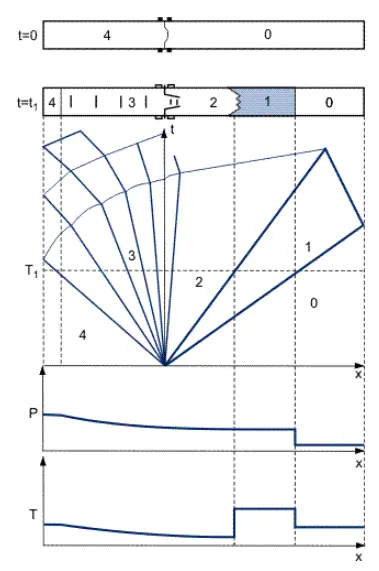
A high-temperature supersonic gas flow is initiated in a shock tube as a result of rupture of a diaphragm separating two gases in high-pressure and low-pressure chambers. An unsteady rarefaction wave passes into the "driver" gas in the high-pressure chamber with a velocity a few kilometers per second. This results in the drivers’ gas flowing into the low pressure gas, pushing the gas in the low pressure chamber ahead of it. The shock wave propagates in the low-pressure chamber ahead of this flow of the studied gas. The velocity of the driven gas flow is equal to that of the driver gas flow. The wave (x − t) pattern, the schematic of the shock tube, and distribution of pressures p and temperatures T along the tube axis are presented in Figure 1. The parameters are denoted by 0 in the low-pressure chamber of the shock tube, 1 behind the incident shock wave, 2 behind the contact surface, 3 in the rarefaction wave, 4 in the high-pressure chamber, and 5 behind the reflected wave. In order to generate a shock wave with the specified pressure ratio p1/p0 in a shock tube, it is necessary to provide the pressure ratio p4/p0 over the shock tube diaphragm. According to this, shock tubes can be devided into four groups.
(1) Shock tubes with an inert gas in the high-pressure chamber. In this case a driver gas is hydrogen or helium at a pressure ranging from several to a hundred atmospheres and of ambient initial temperature. For pressures in the low-pressure chamber from 1 to 100 mmHg, the shock wave velocities range from 0.5 to 6 km/s. The temperature behind the shock wave is from 1000 to 10,000 K. The length of the high pressure gas zone, depending on the tube length and the shock wave velocity, is from several centimeters in laboratory tubes, whose length does not exceed 10 meters, to a meter in test shock tubes 50 to 100 meters long.
(2) Shock tubes with an explosive in the high-pressure chamber. In this case, in the high-pressure chamber, a hydrogen-oxygen-helium mixture or a solid explosive charge are used to increase the initial temperature of a driver gas. The gas temperature behind the shock wave amounts to 20,000 K in an inert gas and 15,000 K in a dissociating gas.
(3) Electrically driven shock tubes. These are tubes in which a discharge chamber with discharge-heated gas is used instead of the high-pressure chamber. Electrically driven shock tubes are designed with and without diaphragms because the parameters of the driver gas increase sharply as a result of discharge. In these shock tubes the velocity of the shock waves varies from 10 km/sec at initial pressures of several millimeters Hg to 100 km/sec at initial pressures fractions of a millimeter Hg. Gas temperature reaches a few tens of thousands of degrees.
(4) Shock tubes with shock wave enhancement. Shock tubes in this category use for shock wave enhancement the interaction of waves arising in transition of a shock wave to sections with different pressure and cross section, the category also includes shock tubes with two diaphragms.
Pre-processor
Geometry & Case Setup
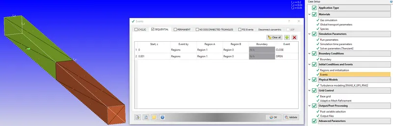
As seen in the following picture, two regions were considered to have O2 and N2 with a 6:1 pressure relationship, starting from 0s as closed regions and at 0.001s the regions were open beginning a convergence process that over a small period of time temperature, velocity, pressure and turbulence will be greatly affected.
Postprocessing
Steady state cases
Paraview
The following images show the contours asked for, for analyzing and seeing the results.
Velocity

Temperature

Converge plots
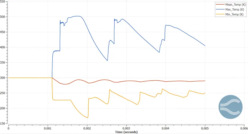
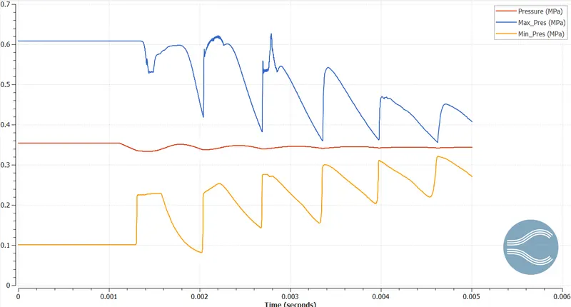
In the following temperature and pressure plots it can be seen that both have the starting 0.001 s before having a great divergence of values that as expected of all real systems it will result in a convergence of stable ending.
Temperature plot
Pressure plot
Cell count plot
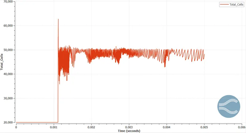
The cell count due to the 50,000-cell restriction it shows a good development in the species variation having a fast and accurate simulation.
Conclusion
The results will be shown in the animations varying through time from 0 to 0.005 seconds having temperature, velocity, pressure and the mesh variation having a refinement along the variation with the fluid species, according to the visualization of the species mesh refinement its able to see the shock wave maintaining itself on the right size of the tube meaning that the higher-pressure specie has a greater surface area to cover and converging pressure in the tube along time.
Having a good visual comprehension of the shock tube problem with the variation of temperature, pressure, and velocity also the benefits of having a great mesh generation throughout time according to a specific variable which in this case is species, as the las simulation for the Prandtl-Meyer shock wave, this simulation is applied to the mechanical-thermal and aerodynamic design for aircrafts, planes according to the supersonic and subsonic environments and the air properties which and engineer have to take into matter for a great design.
VIDEO TEMPERATURE
VIDEO VELOCITY
VIDEO SPECIES
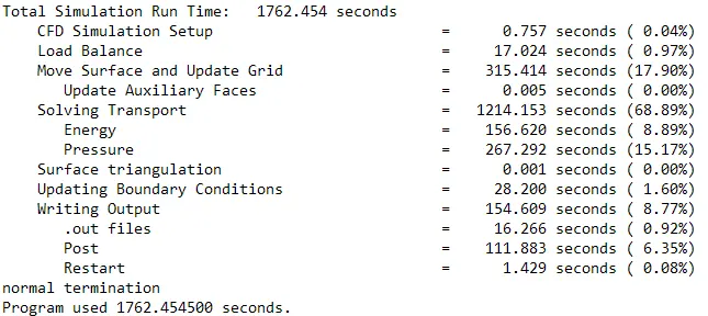
TIME ANALYSIS SHOCK TUBE
References