Week 7: Shock tube simulation project

Introduction:

Shock tubes are used to replicate and direct blast waves to simulate actual explosions and their effects in a scaled down geometry. They are used to investigate compressible flow phenomena and gas-phase combustion reactions. A shock wave inside a shock tube may be generated by a small explosion (blast-driven) or by the gradual buildup of high pressures which cause diaphragm(s) to burst and a shock wave to propagate up and down the shock tube in the low pressure and high pressure region.

 

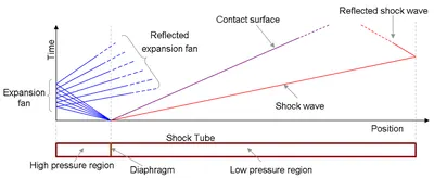
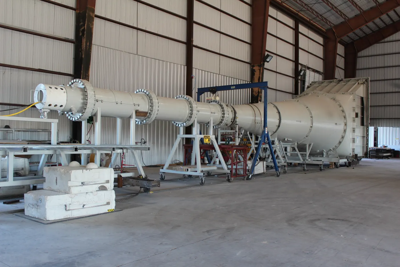
The diaphragm at the middle of the chamber suddenly bursts open under predetermined conditions to produce a wave propagating through the low and high pressure section. But, in a short interval of time, compression waves coalesce to form the shock wave which propagates in the low-pressure section. The generated shock wave as a result increases the temperature and pressure of the gas and induces a flow in the direction of the shock wave. The stationery low-pressure gases experience a rise in pressure and temperature due to the arrival of shock waves. Both the expansion fan and the shock waves are reflected to and froth  from the closed ends of the tube. The induced flow in the direction of the shock wave is at lower velocity than the lead wave. The strength of the shock wave and expansion fan depends on the initial pressure ratio across the diaphragm and physical properties of the gases in the sections.

Objective : 1.Transient simulation of a shock wave inside a shock tube by the aid of Converge CFD software.

2. To extract how the pressure and temperature behaves in the regions of entire flow domain through paraview.
3. Assigning AMR with SGS parameter and see the effect

Geometry: A box of length 0.2m, with breadth and height of 0.01m, is modeled with two regions as shown below.  The whole flow domain is divided by two wall boundaries which represents two regions, high pressure and low pressure along with Boundary flagging. The diaphragm is removed as it is not possible to break the diaphragm by the aid of the software.

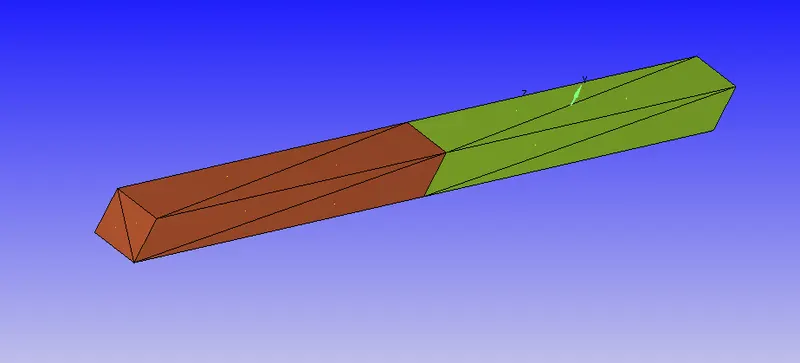
Region Green - High-Pressure Region (N₂ gas)

Region Brown - Low-Pressure Region (O₂ gas)

Both regions are operated by events to act as a diaphragm and it’s sudden break creating an blast driven explosion to obtain the shock during the simulation and to separate the regions before the explosion (i.e., the opening of the diaphragm).

Meshing: The below figure shows the AMR applied in the Mesh at the last time step

 

Case Setup:

Physical Setup: General :Transient  simulation ~ Pressure Based  

Model -RNG k-ε

Gas Species : O₂ , N₂ .

Solver : Transient solver , Fully Hydrodynamic.

Gas flow solver : Compressible with Momentum , Energy turned on 

Simulation Time parameters

Simulation Time 0 to 0.003 s

Initial Time-step : 1e-9s

Minimum Time-step 1e-9s

Max time-step 1s.

Solver scheme : Piso algorithm : Density Based

Boundary Conditions ~walls (slip)

High-Pressure Region ( N₂, 6e5 Pa, 300K)

 Low-Pressure Region ( O₂, 101325 Pa, 300K)

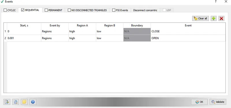
Events:  0-0.001s (close) 0.001-0.003s (open)

Adaptive Mesh Refinement with Base Grid 0.001m

N₂ species SGS - 0.001

Cell count :

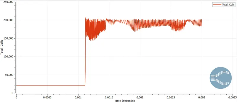
The below plot shows the variation of mesh sizes as a function of time during the entire simulation of 0.003 seconds. The sudden shooting up of cell count at 0.001 second is the diaphragm bursts i.e the two regions( H.P and L.P regions) couples and simulation starts. That very moment  the high pressure region pushes the low pressure region  as a result the AMR SGS activates. The sudden decrease in mesh size is when the reflected wave due to the oscillatory behaviour of pressure difference, the L.P region  pushes the H.P region back and the cycle continues until the pressure difference dampens.

Post processing Results :

Mass fraction N₂ Contour : As the diaphragm breaks the (high pressure region )N₂ pushes the low pressure region(O₂) then the low pressure region reflects back again and pushes the shock wave towards N₂ region. In such a way a back and froth movement takes place, as a result  the waves have different pressures and temperatures through the simulation time.

Mass fraction of O2

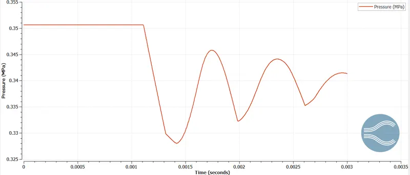
The High pressure region is 600 kPa and as seen from  the plot below,  the simulation never reaches that pressure. As soon as the diaphragm breaks at 0.001 seconds the pressure  shoots upto 360 kPa and at the very next moment the high pressure region pushes the low pressure region and as the pushing from H.P to L.P and vice versa goes on which means that as the reflected wave is genberated after the first push from H.P to L.P ,the pressure slightly drops as we can see from the plot and when the reflected wave is generated on the low pressure region to push towards the high pressure region, the pressure rises.

Total Pressure variation in the flow domain:

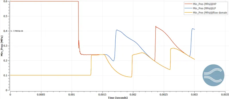
Variation of Mean Pressure in all the flow domains:(High Pressure region, Low pressure region and the complete flow domain)

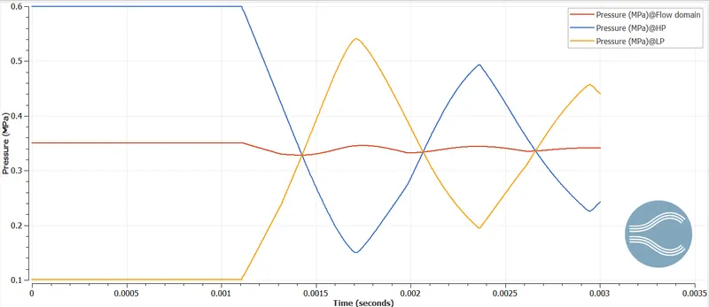
Variation of Total Pressure in all the flow domains:(High Pressure region, Low pressure region and the complete flow domain)

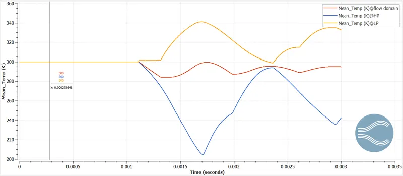
Similarly with temperature plot a continual oscillation of temperature value takes place. We can see that the highest temperature is at the high pressure region and as shock propagates it increases the temperature of lower region which is a result of significant pressure difference. The plot signifies average total temperature for both regions.

#anim for temperature

Total avg Temperature variation in the flow domain:

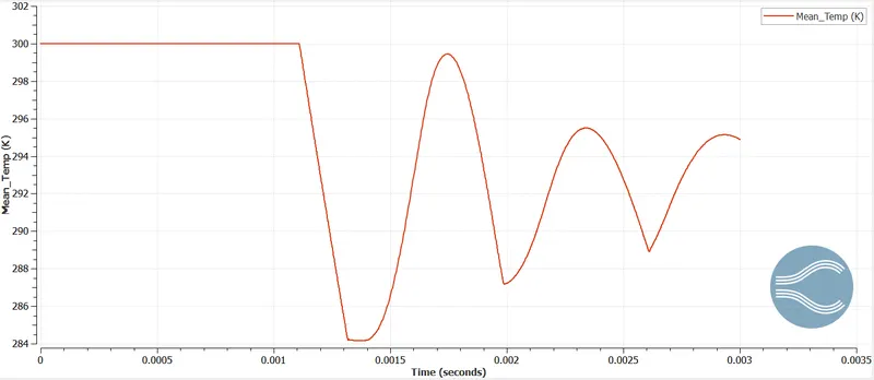
Variation of Mean Temperature in all the flow domains:(High Pressure region, Low pressure region and the complete flow domain):

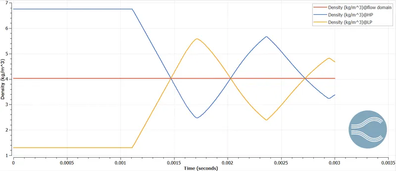
Density variation in all the flow domains:

Velocity animation

Discussion and Analysis:

The process of generation of shock and expansion waves continues till the difference in pressure in the whole domain nullifies/damps which can be seen if ran for more time steps  for which the assigning of  AMR whose sole purpose is to refine  the mesh in the wavefront until the rate of change of concentration of N₂ is below the SGS value. The diaphragm breaks at 0.001s which is activated by events. As soon as the diaphragm breaks at 0.001 seconds the pressure  shoots upto 360 kPa and at the very next moment the high pressure region pushes the low pressure region and as the pushing from H.P to L.P and vice versa goes on. The shock waves are reflected when the gases in the Low-pressure region are compressed and the pressure in the Low pressure region is higher than the Shock front. This oscillating behaviour is observed until the pressure difference damps out.