SHOCK TUBE SIMULATION USING CONVERGE CFD
Aim: To setup and run shock tube simulation in Converge CFD
1. Study the Pressure and Temperature variations due to the shock wave
2. Study how cell count changes due to mixing of two different species.
Shock Tube setup and working:
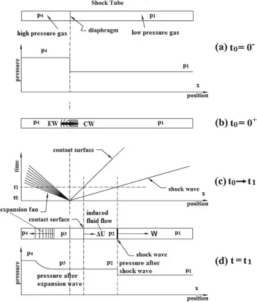
The shock tube is a simple duct closed at both ends. A diaphragm divides this duct into two compartments called as driver (high pressure) and driven (low pressure) sections. These two sections are separated by a metal diaphragm. A high pressure driver gas reservoir is connected with the driver section. However a vacuum pump is connected to the driven section to arrive at the accurate driven section pressure. Pressure sensors are generally mounted along the driven tube for pressure measurement. A shock wave inside a shock tube may be generated by a small explosion (blast-driven) or by the buildup of high pressures which cause diaphragm to burst and a shock wave to propagate down the shock tube (compressed-gas driven).
In our case we are implementing compressed-gas driven method. By slowly increasing the driver gas pressure for a given driven pressure until the diaphragm gets ruptured. Burst of the diaphragm creates a compression waves which propagate in the driven section and expansion waves traversing in the driver section. In a short interval of time, compression waves coalesce to form the "Shock wave" which propagate in the driven section. The stationary low pressure driven gas raises its pressure and temperature on arrival of the shock wave. Driver gas at the same time encounters the expansion in the presence of expansion waves. The contact surface moves in the driven section which separates the driver and driven gases and provides the position of diaphragm. Expansion waves do not coalesce, so they form an "Expansion Fan". Both the expansion fan and shock reflect from the closed ends of the shock tube. Reflected shock cancels the motion of the driven fluid initiated by the primary shock, thus providing more resistance against mixing. Collision and boundary layer effect results in small pressure loss, as the energy gets transferred in the form of waves.
Uses of Shock Tube:
The shock tube is an instrument used to replicate and direct blast waves at a sensor or a model in order to simulate actual explosions and their effects, usually on a smaller scale. Shock tubes can also be used to study aerodynamic flow under a wide range of temperatures and pressures that are difficult to obtain in other types of testing facilities. Shock tubes are also used to investigate compressible flow phenomena and gas phase combustion reactions
Shock tubes are used to replicate and direct blast waves in order to simulate actual explosions and their effects on a smaller scale. Moreover, they are used to investigate compressible flow phenomena and gas-phase combustion reactions. A shock wave inside a shock tube may be generated by a small explosion (blast-driven) or by the buildup of high pressures which cause diaphragm(s) to burst and a shock wave to propagate down the shock tube (compressed-gas driven). The burst of the diaphragm creates a compression wave that propagates in the low-pressure section and expansion waves traversing in the high-pressure section. However, in a short interval of time, compression waves coalesce to form the shock wave which propagates in the low-pressure section. The stationery low-pressure gases experience a rise in pressure and temperature due to the arrival of shock waves as shown in the figure below. Both the expansion fan and the shock waves are reflected from the closed ends of the tube. Reflected shock counters the motion of the low-pressure section initiated by the primary shock. The strength of the shock wave and expansion fan depends on the initial pressure ratio across the diaphragm and physical properties of the gases in the sections.
In a Diesel engine, diesel in injected at a high pressure in compressed air which is at a relatively lower pressure. The compressed air is at a higher temperature because it is compressed. Now because of this pressure and temperature difference, the diesel fuel starts to mix with the air. Ignition delay in a diesel engine is the time interval between the start of injection and start of combustion. This delay period consists of physical delay and chemical delay. Both of them occur simultaneously. Physical delay is due to the vaporization, atomization and mixing of air-fuel and chemical delay is due to pre-combustion reactions. To reduce the unburnt fuel and CO pollutants, the mixing of fuel with air is very important and to reduce NOx, the method adapted in modern engines is to reduce the ignition delay. In the shock tube simulation we get to know how much time it takes for the two different species to mix and how the shock wave affects the pressure and temperature domain, for a given pressure difference.
Case Setup
1. Application Type: Time Based
2. Gas Simulation, Equation of State = Redlich-Kwong (all default settings)
3. Global Transport Properties: All defaults values.
4. Species: Gas: O2 and N2
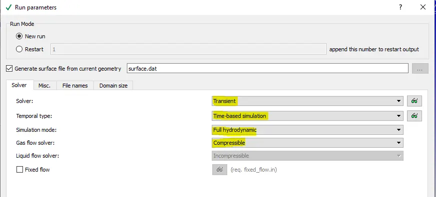
5. Run Parameters
Solver settings: Transient, Time based simulation, Full Hydrodynamic and Compressible.
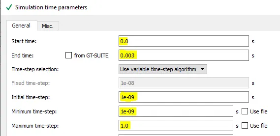
6. Simulation Time Parameters
Start time: 0 seconds
End time: 3 milli seconds
Initial and Minimum time step: 1e-9 seconds
Max time step: 1 second
7. Solver Parameters: Default settings
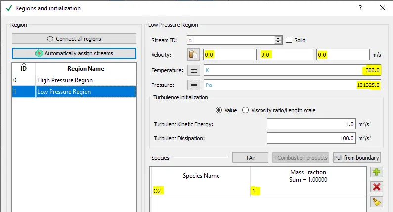
8. Regions and Initializations
Two regions
High pressure Region with 300K temperature, 6 bar pressure, species as N2 (mass fraction = 1.0)
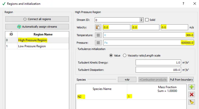
Low pressure Region with 300K temperature, 1 atm pressure, species as O2 (mass fraction = 1.0)
9. Boundary Conditions
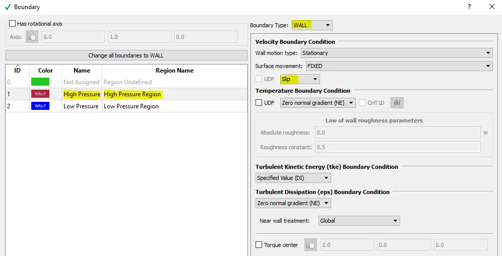
High Pressure boundary in high pressure region. Boundary type as Wall, Velocity boundary condition as slip
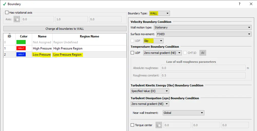
Low Pressure boundary in low pressure region. Boundary type as Wall, Velocity boundary condition as slip
10. Turbulence Modelling
Turbulence model: RNG k-epsilon
All settings default.
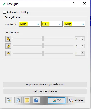
11. Base Grid Size
Grid Size = 0.001 m or 1 mm
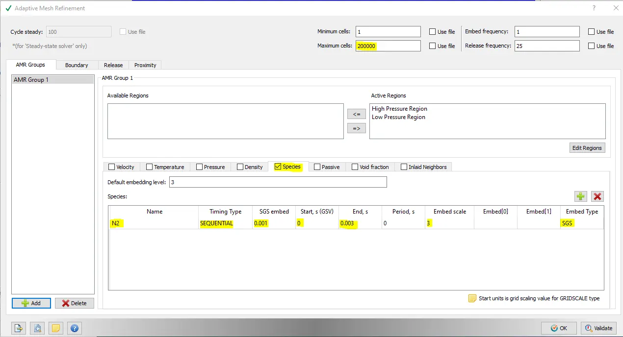
12. Adaptive Mesh Refinement
Species AMR with N2 species, embedding level = 3, SGS parameter = 0.001, embed scale = 3 and max cells = 200000
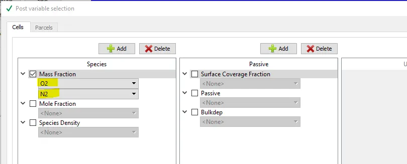
13. Post Variable selection
Include O2 and N2 species under mass fraction
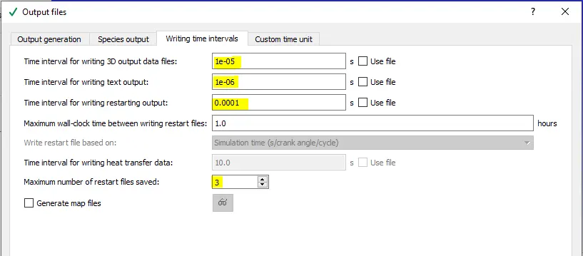
14. Output Files
Set the time interval for writing 3D output as 1e-5 to create a smooth animation and text output as 1e-6 to create a smooth plot.
Set the time interval for restarting output as 0.0001 so there are atleast 30 restore points during the entire simulation.
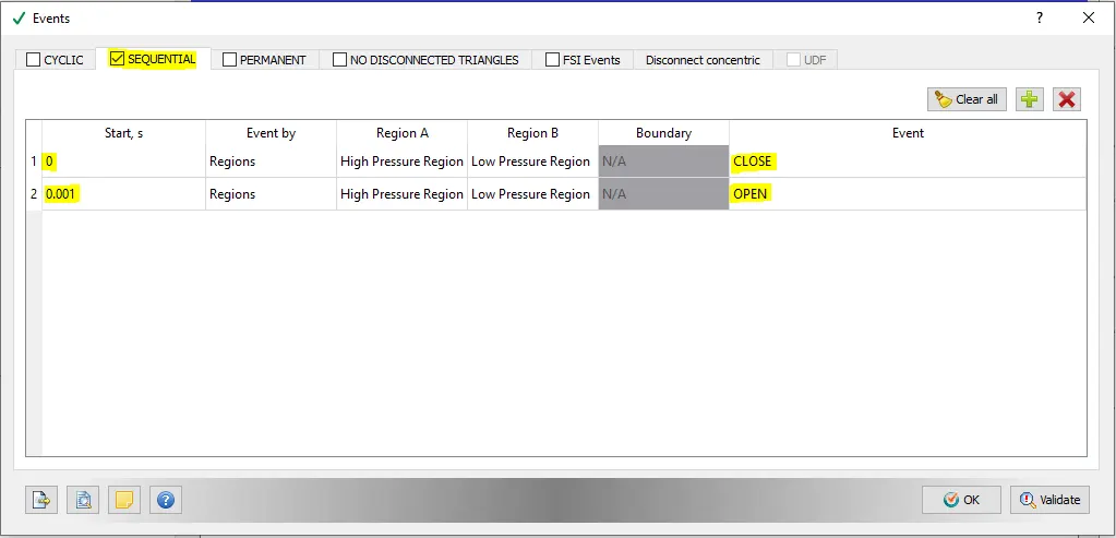
15. Events
Events type as Sequential. Add 2 events
1. At 0 seconds time the diaphram between high pressure region and low pressure region should be closed.
2. After 1 milli second time the diaphram between high pressure and low pressure region should be open.
Results of Simulation
Mesh
at 0th time step

at final time step

Mesh (Animation)
From the above video we can see that the mesh refinement takes place near the N2 - O2 interface and this mesh refinement keeps changing as the shock propogates back and forth.
Pressure Plot
Observation from the above plot
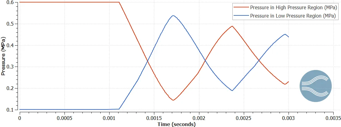
1. As the diaphram is removed the pressure in high pressure region drops from 6 bar to close to 1.5 bar in just half a millisecond (0.0011 to 0.0017 seconds) and then keeps fluctuating. The magnitude of the fluctuations in pressure is (6-1.5)/2 = 2.25 bars in just 0.0006 seconds which is tremendous.
2. Similarly, in the low pressure region the pressure increases from 1 atm to 5.2 bars in just 0.0006 seconds (0.0011 to 0.0017 seconds) and then keeps fluctuating.
3. The magnitude of the pressure peaks keeps decreasing with time which indicates that the shock wave will die out after a couple of milli seconds. Since we ran the simulation only till 3 milliseconds we are unable to see the shock waves die.
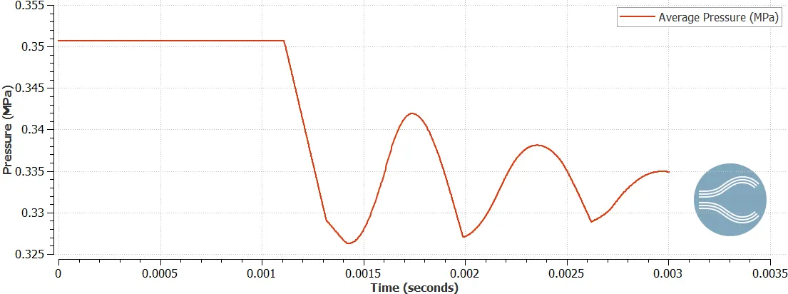
Observe how the pressure fluctuates in the entire domain as well as in the high pressure and low pressure regions due to the shock wave.
Pressure Contour Plot (Animation)
Observation:
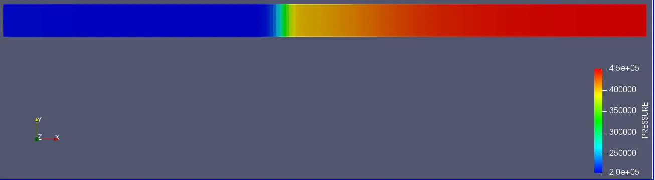
From the above animation we can see that how the shock wave travels in a one direction and when it reaches a dead end it gets reflected back and travels in the opposite direction and the process repeats untill it dies out.
Temperature Plot
Mean Temperature fluctuation
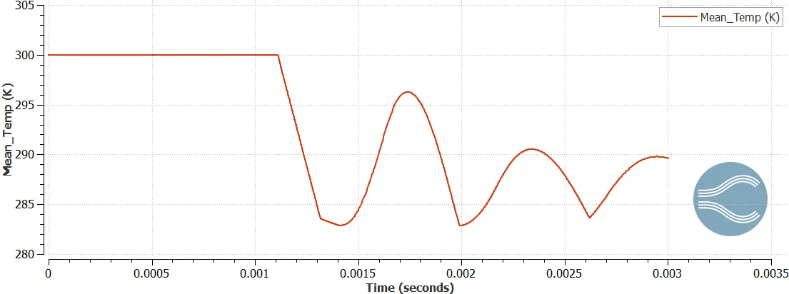
Mean Temperature fluctuation in High Pressure and Low Pressure regions
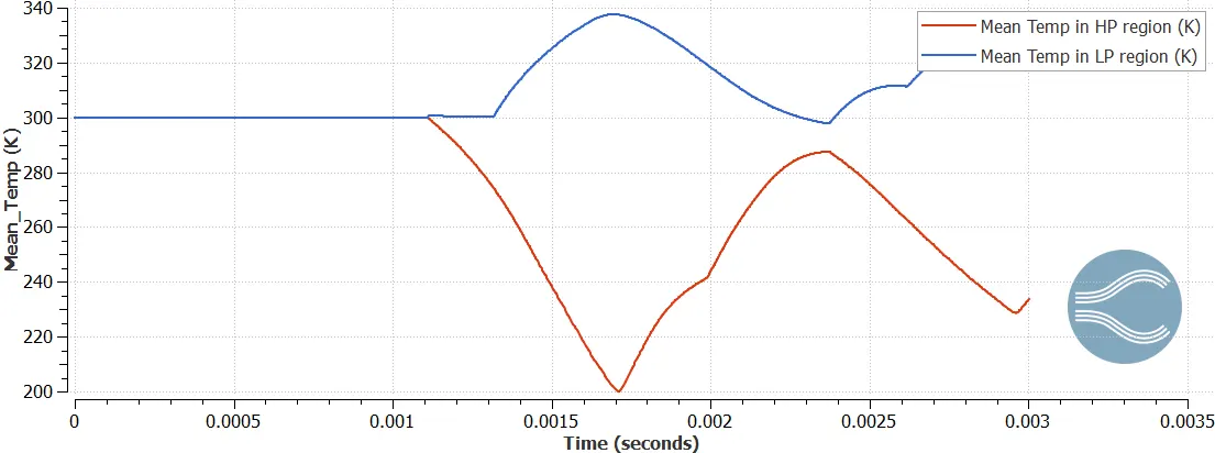
Observe in low pressure region, the mean temperature drops from 300 K to 200 K in just a half millisecond.
We can see how the mean temperature fluctuates in a fraction of a milli second. This fluctuation are due to the shock wave.
Temperature Contour Plot (Animation)
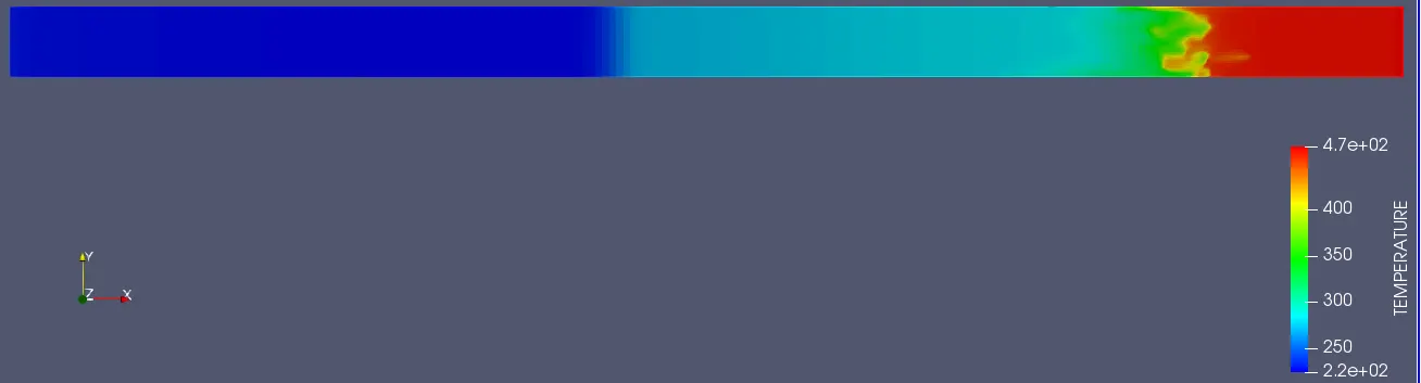
Observation:
From the above animation we can see that how the shock wave travels in a one direction and when it reaches a dead end it gets reflected back and travels in the opposite direction and the process repeats untill it dies out.
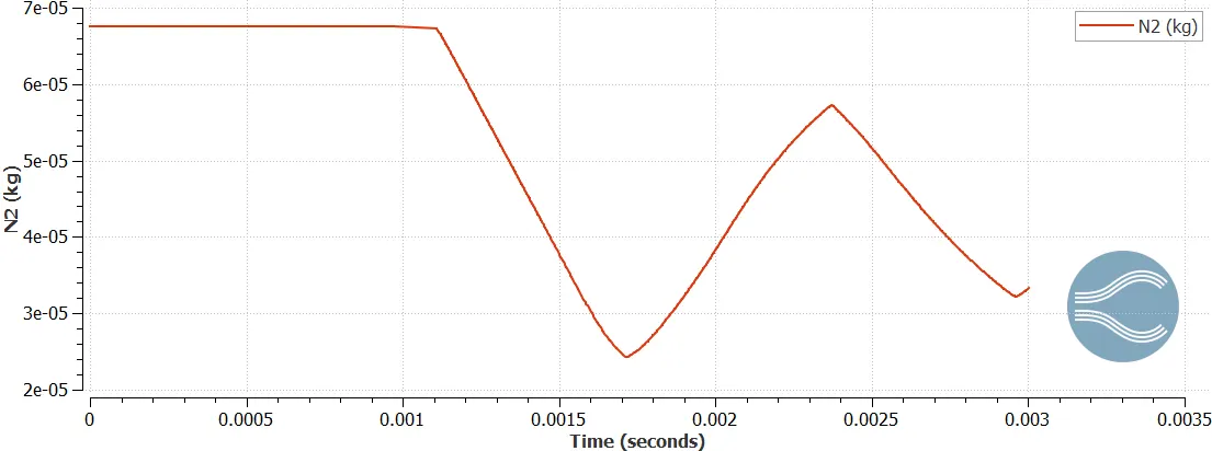
Mass of N2 in high pressure region as a function of time
Mass of O2 in the Low pressure region as a function of time
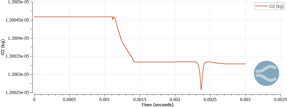
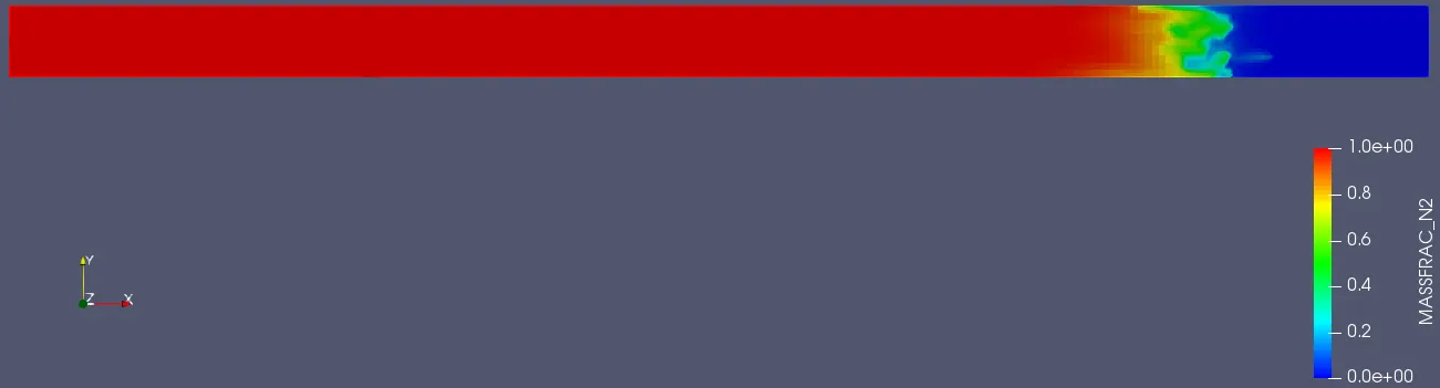
Observation: As the time progresses the N2 mass in high pressure region decreases and O2 mass in the low pressure region also decreases. This indicates how the two different species mixes with one another as a function of time.
Mass Fraction (N2) Animation
Mass Fraction N2 Plot at final time step
Cell Count as a function of Time
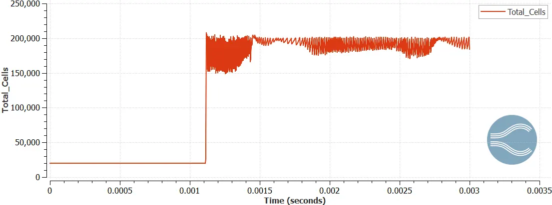
As we can see from the above plot that as the diaphram is opened the N2 gas at high pressure started mixing with the O2 gas at low pressure. Adaptive mesh refinement was used by converge at the interface of N2 and O2 gas when both the gases started mixing and hence there was a sudden rise in number of mesh cells when the diaphram was opened.
Shock tube velocity variation animations :
white colour vectors indicate the high pressure region intially we have taken and black colour vector indicate the low pressure region
Conclusion :
A Transient shock tube simulation was setup and run in Converge. Shock propogation and reflection was studied from the Pressure and Temperature history in the entire domain. The effect of adaptive mesh refinement on the number of cells as a function of time was studied.