Shock tube simulation using Converge CFD

Objective:

1. Setup a transient shock tube simulation.
2. Plot the pressure and temperature history in the entire domain.
3. Plot the cell count as a function of time

Introduction

The shock tube is an instrument used to replicate and direct blast waves at a sensor or a model in order to simulate actual explosions and their effects, usually on a smaller scale. Shock tubes (and related impulse facilities such as shock tunnels, expansion tubes, and expansion tunnels) can also be used to study aerodynamic flow under a wide range of temperatures and pressures that are difficult to obtain in other types of testing facilities. Shock tubes are also used to investigate compressible flow phenomena and gas-phase combustion reactions.

A simple shock tube is a tube, rectangular or circular in cross-section, usually constructed of metal, in which gas at low pressure and gas at high pressure is separated using some form of a diaphragm. The diaphragm suddenly bursts open under predetermined conditions to produce a wave propagating through the low-pressure section. The shock that eventually forms increases the temperature and pressure of the test gas and induces a flow in the direction of the shock wave.

Geometry

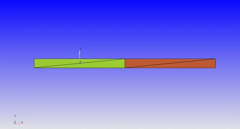
The STL file is imported in converge studio. Boundaries are flagged according to the simulation requirement.

Case setup

Species; O2, N2

Solver: Transient

Navier- stokes solver type: Density-based

Simulation mode: Full hydrodynamic

Gas flow solver: Compressible

Boundary conditions

All the boundaries are given as stationary wall BC (Slip BC)

Regions

High pressure

• Species: N2
• Pressure=600000 Pa
• Temperature=300K

Low pressure

• Species: O2
• Pressure=101325 Pa
• Temperature=300K

Events

An event is created for simulating the bursting diaphragm, In the beginning, the high pressure and low-pressure regions are disconnected. After 0.001s it became connected and mixing takes place.

Simulation time parameters

Start time=0 s

End time=0.003 s

Initial time step= 1e-9 s

Minimum time step= 1e-9 s

Maximum time step= 1s

Output files

The time interval for writing 3D output files=1e-5 s

So the solver writes a 3D output files after every 1e-5 seconds.

Mesh

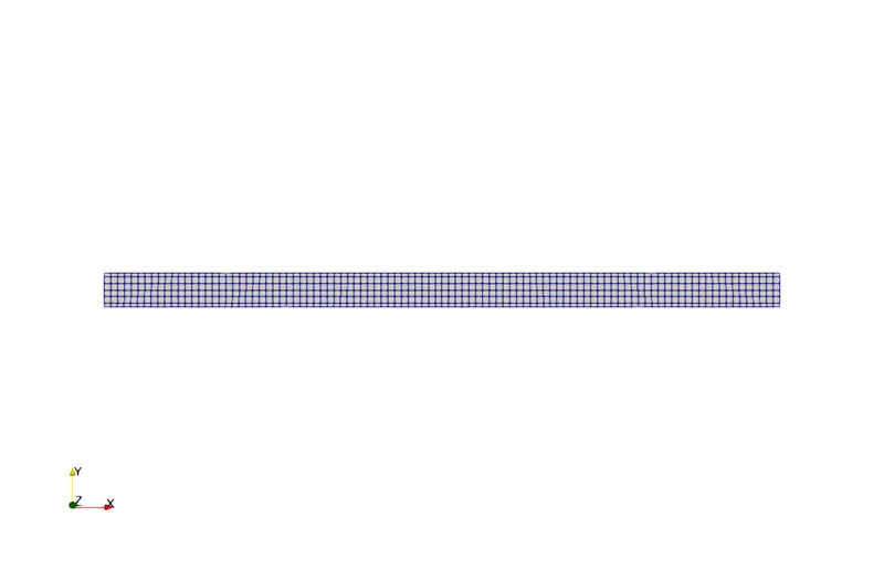
Mesh generated without AMR is shown in the above figure.

Base grid =0.002 m

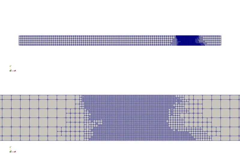
In order to obtain better results, a species based Adaptive mesh refinement is used. The AMR is based on N2 species with an embedding level of 3. The AMR generated in the last timestep is shown below,

Post-processing and results

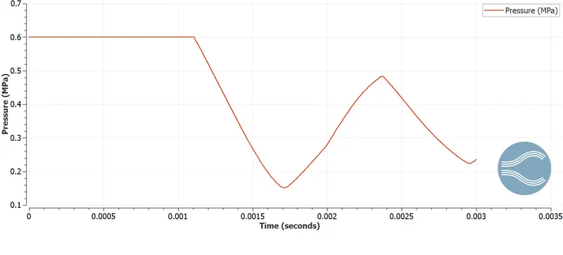
Pressure (High-pressure region)

Pressure (Low-pressure region)

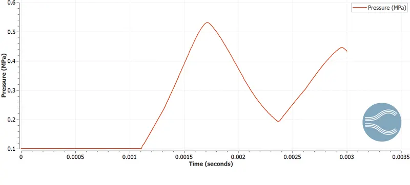
When the diaphragm burst at 0.001s mixing takes place. The high-pressure gas or driver gas (N2) rushes to the low-pressure region. Due to this pressure in the high-pressure region decreases and pressure in the low-pressure region increases.

Temperature

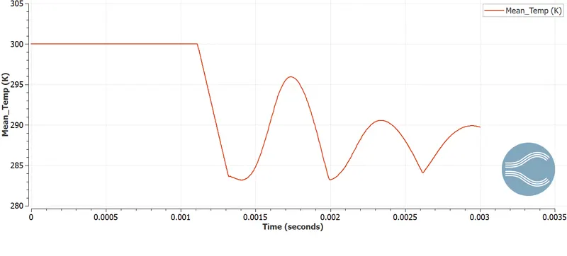
Temperature is constant till 0.001s, the temperature is the same as the initial temperature (300K). When the mixing takes place mean temperature decreases.

Total cell count

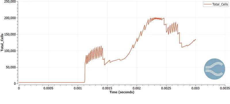
In the beginning, two regions are disconnected no mixing takes place, After 0.001s the diaphragm bursts and the high-pressure gas (N2) rushes to the low-pressure region. In this time adaptive mesh refinement occurs with species N2 and cell count increases. The cell count for the base grid is 2500 and it increases up to 200000 when adaptive mesh refinement takes place. After sometime when the system approaches equilibrium the cell count decreases.

Animation

The animation of velocity and mass fraction of N2 is shown in the above video, In this, we can see the shock wave forming after 0.001s.

Conclusion

1. The AMR gives better results with a coarser base grid size, it increases the cell count initially, and when the system approaches equilibrium cell count decreases.
2. When the diaphragm bursts, driver gas rushes to the low-pressure region (driven gas) The bursting diaphragm produces a series of pressure waves, each increasing the speed of sound behind them so that they compress into a shock propagating through the driven gas. This shock wave increases the temperature and pressure of the driven gas and induces a flow in the direction of the shock wave but at a lower velocity than the lead wave. Simultaneously, a rarefaction wave, often referred to as the Prandtl-Meyer wave, travels back into the driver gas.