Shock tube simulation project

Aim:

This particular project aims at obtaining a transient simulation of flow in a shock tube.

Governing Equations:

The simulation is run on the basis of the Navier Stokes equations. The NS equation consists of three momenta, one continuity, and one energy equation. The energy equation is solved only during the time where there is a heat transfer taking place. This is done so to reduce unnecessary computational time.

Objective:

The objective is to study the behavior of fluid inside a shock tube. Another objective would be to understand the use of events in the simulation arena.

The workflow involves:

1. Importing a geometry of the shock tube.
2. Flagging the boundaries starting from the flow into the model and the fluid exiting from it.
3. Creating the required case setup and setting up parameters according to the requirements.
4. Transporting the input files and running the simulation.
5. Convert the obtained 3D files into a corresponding viewable form.

Obtaining the contours and animation and drawing results from them using a 3D viewing platform such as ParaView.

The case setup:

The case was setup with a different approach here. The body was divided into just two boundaries, one with higher pressure and another with a low-pressure boundary. Once the boundary flagging is finished, the case setup is started, starting with time-based as the application type. Air is selected as a gas mixture. Global transport parameters were selected to be the default with the Prandtl number being 0.9 and Schmidt number being 0.78.

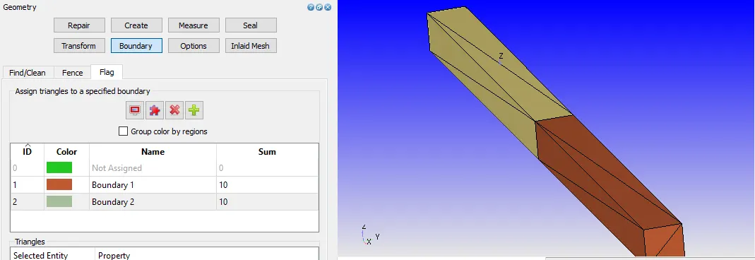
Figure1. Screenshot involving boundary flagging window during a shock tube simulation

The simulation was run with a base mesh size of 4mm. The solver was selected to be a transient solver. The simulation was run for 5ms with an initial time step of 1e-7seconds. The solution was obtained using the NS equation. The solver scheme was selected to be PISO. PISO stands for Pressure Implicit with Splitting of operator. Turbulence modeling was run according to the RNG k-ε equation.

The high-pressure boundary was set up with a pressure of 6bar and the low-pressure boundary was set up to have 1bar. The difference between the pressure drives the flow from the inlet to the outlet.

Another important setup would be the events. Events are used when we have to have a sequence of process that needs to take place. In this problem, we need to replicate the flow through a diaphragm. The flow initially would not flow due to the presence of the diaphragm and later due to the high pressure, breaks, and the flow takes place. This sequence is replicated using the events. At time 0 seconds, the flow would not take place and after time 1ms, the flow would rupture the diaphragm as seen in Figure below.

The AMR was set to vary in accordance with the species. Hence the mesh followed the changes taking place with the N2 species. The timing was set to be permanent with SGS embed level of 0.001.

Coming to the output files, the 3D output files were made to write at an interval of 1e-5 and the text output was written at every 1e-6th second.

Results and Figures:

Since the adaptive mesh refinement was chosen, the number of cells was not constant which is clearly visible in the plot below. The simulation initially starts with a cell count of almost zero until the diaphragm ruptures. Once after the event, the cell count observes a meteoric rise in the count with an increase to around 15000 cells. The cells somewhat stay constant from 1.5ms to 2ms and then again observe a rise up to 30000 cells with a peak of around 32000 cells. This can be attributed to the rebound that takes place within the tube and also due to the mixing of the N2 and O2. A look at the surface with edges after the rupture of diaphragm is seen in the Figure below that shows the AMR following the flow of N2 and refining the number of cells at that local position.

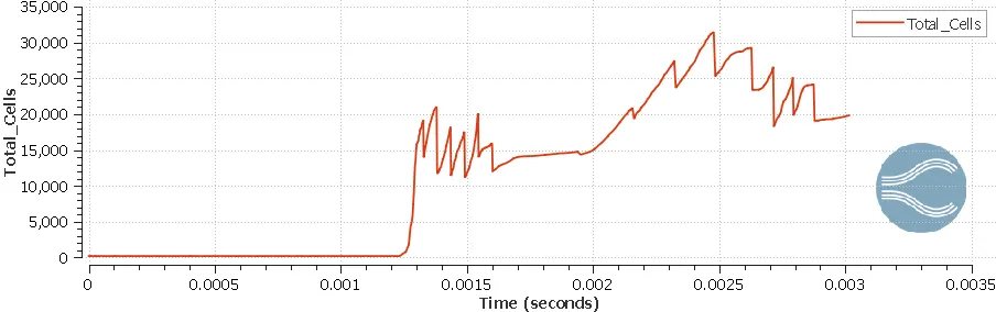
Figure2. Plot of cell count variation obtained during a shock tube simulation

Figure3. Plot of surface with edges obtained during a shock tube simulation

The pressure plots were obtained as seen below. The max pressure was observed to be around 6bar as set during the case setup. The 6bar pressure is maintained up until the 1ms mark after which the pressure observes a huge variation in its value due to continuous mixing and separation of N2 and O2 that occurs because of the rebounding. The pressure reaches a minimum of 1 bar as seen in the Figure below. The average is around 3.5 bar and observes an immediate drop in pressure once after the diaphragm is broken.

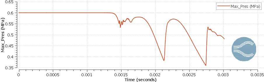
Figure3. Plot of Max pressure (MPa) obtained during a shock tube simulation

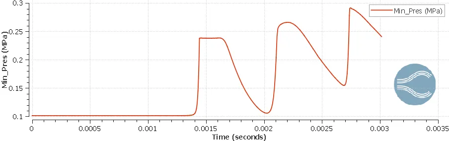
Figure4. Plot of minimum pressure (MPa) obtained during a shock tube simulation

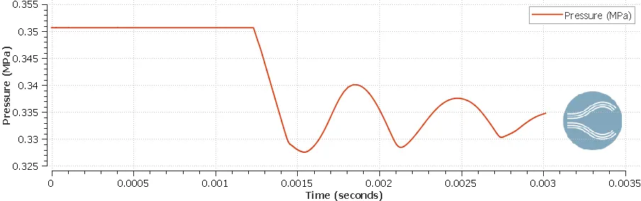
Figure5. Plot of avg pressure (MPa) obtained during a shock tube simulation

The temperature is observed to be varying from a maximum of 480K to a minimum of 190K as seen in the plots below. This huge variation is again in accordance with the shock which arises due to the pressure variation that occurs inside the tube. The peak and dropping nature of the curve is due to the rebound of the fluid across the tube time and again.

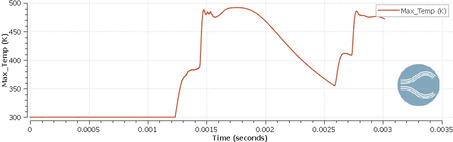
Figure6. Plot of Max temperature (K) obtained during a shock tube simulation

Figure7. Plot of Max temperature (K) obtained during a shock tube simulation

Conclusions:

The results obtained are physical in nature which means the plots and the animation behave according to the way the case was set up. The events dock ran exactly according to the setting with the diaphragm rupturing at 1ms. This problem provides a very good sight of the shock that might occur in an engine cylinder with the fluid being the air and fuel. The link for youtube would be https://youtu.be/ib-ecZwZinI