FULL HYDRO case set up (PFI)

Aim:

The project aims at obtaining a full working PFI engine with the necessary spray, combustion, and spark models completely set up.

Introduction:

Setting up a working engine initially requires importing a CAD file of the component from another environment to the CONVERGE studio. The CAD is then cleaned up by using the repair and patch options present in the software. This geometry was later flagged and the case set up was carried out step by step as mentioned in the coming sections.

Governing Equations:

The simulation is run on the basis of the Navier Stokes equations. The NS equation consists of three momenta, one continuity, and one energy equation. The energy equation is solved only during the time where there is a heat transfer taking place. This is done so to reduce unnecessary computational time.

Objective:

The objective is to obtain a clean surface for the given PFI engine and later to set up a no hydro simulation.

The workflow involves:

1. Importing the PFI engine .cvg file.
2. Running the diagnosis to find out the errors in the geometry.
3. Cleaning the geometry step by step eliminating one surface error at a time.
4. Flagging the boundaries starting from the flow into the model and the fluid exiting from it.
5. Creating the required case setup and setting up parameters according to the requirements.
6. Transporting the input files and running the simulation.
7. Convert the obtained 3D files into a corresponding viewable form.
8. Obtaining the contours and animation and drawing results from them using a 3D viewing platform such as ParaView.

Surface preparation:

The imported file was run for diagnostics and the surface errors as shown in Figure1 appeared. These errors were cleared in a phased manner. The errors could be easily identified with the flagging the boundaries. Hence the boundary was flagged distinctly as seen in Figure2.

The relatively easier corrections were carried out starting from the open edges. Open edges arise when there is a discontinuity on the surface which basically means that there are gaps that need to be filled in. This was done by using the show with a boundary option available in the diagnostic dock window. These were repaired using the patch option available. These patches create the necessary triangles required to complete the surface.

A crucial part of the engine setup would be the valve and its part. The geometry provided had a lot of intersection errors as seen in the figure. A closer look revealed that the valve body was intersecting with the cylinder head and as a result the intersection errors and all the errors that arose. The solution was to push the valves inside the cylinder head to avoid the intersection. Since the valve is at an angle, it’s direction was first found out using the arc normal method that involved choosing any three points on the circumference of the valve. Once after obtaining the required direction, the valves were translated using those coordinates to make sure that the valves were not intersecting the cylinder head. Running the diagnostics again obtained a green checkmark on all errors indicating the geometry is good for case setup.

Case Setup:

The application was chosen to be the IC engine. The boundaries were flagged. The flagged boundaries are as seen in Figure3. To improve the ease and also to maintain proper boundaries, the engine was divided using boundary fences. The valves were divided into the valve stem, valve angle, and valve bottom. It helped in allocating these valves to different regions later on.

The Law of the wall is used for all the boundaries that are set to be a wall. To understand the significance, let us first get to the flow over the wall. The fluid close to the wall experiences high viscosity and as a result the fluid near the wall almost reaches the zero velocity condition. The farther the fluid flows away from the wall, the velocity increases gradually. Predicting wall temperature from the CFD simulation yields a highly inaccurate value because it does not take into account the laminar region involved. The wall Law of the wall includes the behavior of the boundary both in the laminar and the turbulent region. It determines how far the first cell is from the wall. That is y+ distance.

Spray Modeling:

CONVERGE uses Lagrangian modeling or spray modeling for obtaining the spray sequence. For the gaseous solver, converge uses the Lagrangian solver and for the liquid sprays uses the Eulerian model. The fuel after getting sprayed in the engine experiences different kinds of forces. The fuel inside the engine is spherical shaped particles called parcels. These parcels after interacting with air present in the chamber break into primary and secondary parcels. Few other parcels collide with each other and form coalescence. Other parcels, due to the heat inside the chamber, evaporate into their gaseous form. A few other parcels experience the drop drag and lose their shape. The Lagrangian model takes into account all the above-mentioned forces experienced by the parcels. It also considers the effect due to turbulent dispersion.

The modeling is carried out in order to set up the injectors and the volume of spray coming out the injectors. The spray modeling required a detailed setup. In the general section, the parcel was chosen to be distributed throughout the cone. The turbulent distribution model was chosen to be the O’Rourke model since this model suits the gasoline-based simulation.

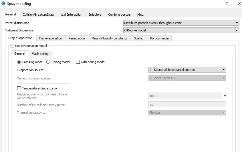
For the evaporation model, the source was chosen to be the base parcel species solved using the Frossling model. The liquid fuel mass fraction for calculating spray penetration was chosen to be 0.95. Which means the penetration length is 95% of the total length of the penetration. The distance measured is not the vertical distance but the distance along the axis of the injector.

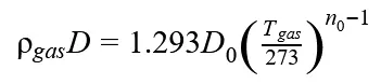
The mass diffusivity constant was calculated using the below-mentioned formula

The collision model was chosen to be the NTC collision model. Collision mesh was used to reduce grid sensitivity. This means that the parcels can now interact with parcels in not only their grid but across the grid. This helps in obtaining a more realistic model.

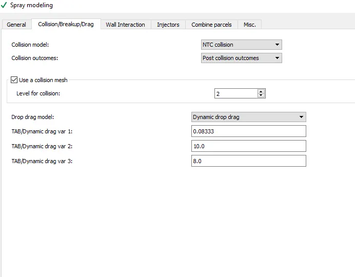
Figure showing the collision model tab available in spray modeling

The interaction between the cylinder wall and parcels were chosen to have a wall film. This means that upon collision with the wall, the parcels would form a thin film on the surface.

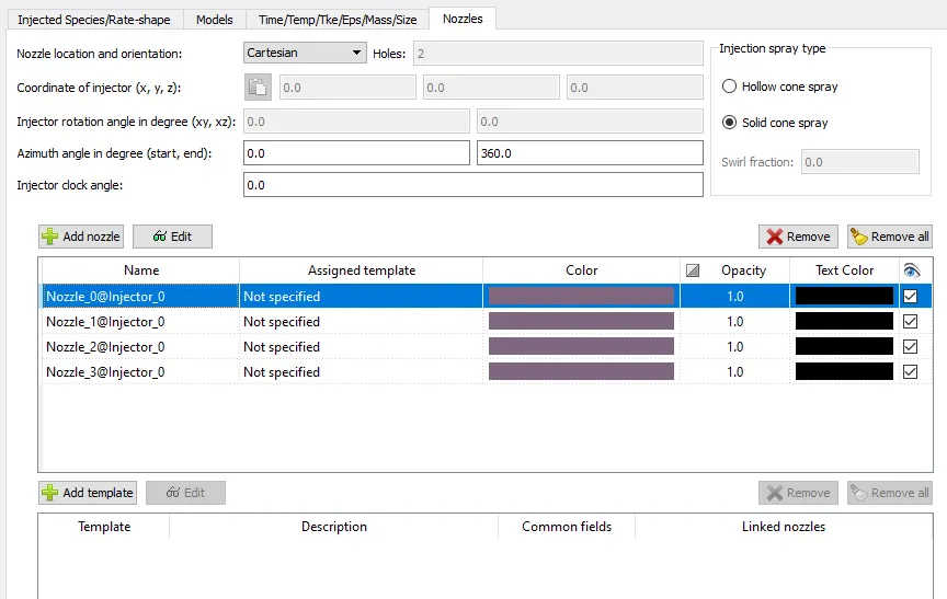
The injectors were set up as follows. The injector was chosen to have four different nozzles. For the injection rate shape profile, points were drawn up the and the plot is as shown in the figure below. The parcel species was selected with a mass fraction of 1.

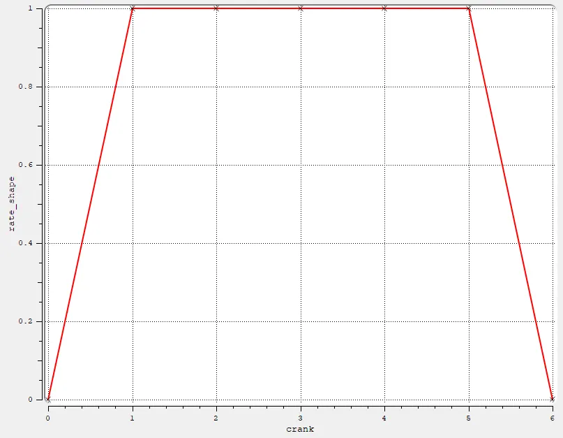
The injector was fitted with four nozzles each having a dia of 250μm and with a spray cone angle of 10 degrees. The location for each of the four nozzles was as provided in the datasheet.

Combustion Modeling:

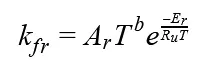
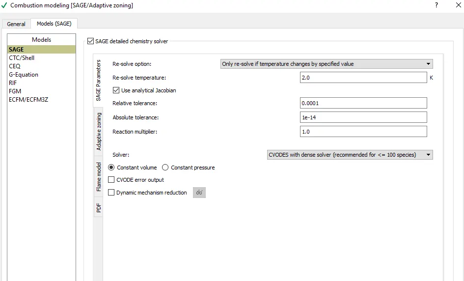
For simulating the combustion, SAGE or the adaptive zoning model was utilized. The calculations of the model are based on the Arrhenius equations which are as given below.

Where,

Kfr is the forward reaction rate

Ar is the pre-exponential factor

b is the temperature exponent

Er is the activation energy

Ru is the universal gas constant

SAGE utilizes both the chemistry solver and the transport solver. The chemistry solver solves the rate of change of species(ODEs) and the transport solver uses the values from the chem solver as the source and uses it to obtain the change in species mass fraction during the length of the combustion.

Solving the chemistry side of the equations is computationally highly expensive since the solver has to produce the rate of change of each species of each cell. Hence to accelerate the process, there are a few things to consider.

To start with, a minimum temperature for the cell can be defined. Doing so would reduce the number of cells the solver has to go through. For complete combustion to take place, each cell should satisfy a minimum fraction of HC’s in them. Hence the solver allows defining a minimum mole fraction for each cell beyond which alone the solver can solve. Another easier solution is to provide a start time just before the start of combustion and end immediately after the combustion. The software also allows defining the solver to work only in certain regions. Since the simulation has to run multiple times, the cell whose temperature increases by a threshold factor can be provided. Another interesting solution is to combine cells to form bins. Bins can be based on two or more variables. This can help reduce computational time by asking the solver to go once per bin instead of once per cell.

Setting up the spark plug:

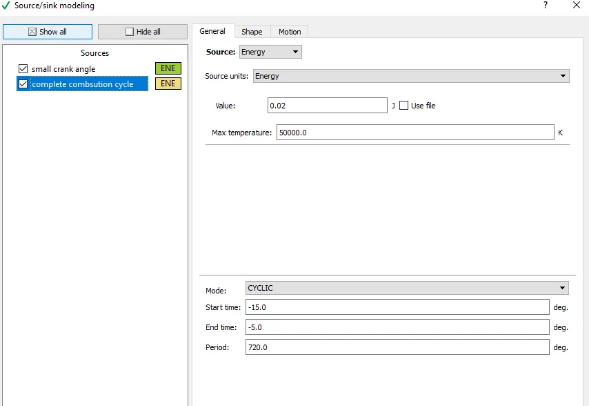
Simulating of the spark plug in converge was performed using source/sink modeling. Spark plugs are devices that help produce the required spark for combustion between their electrodes. The spark generation has three phases in general. The breakdown phase, the arc phase, and the glow phase. During the breakdown, phase is the time when the spark establishes a potential difference between its electrodes. As a result, this phase consumes high energy than the other two phases. The arc phase is the region where the arc is in the process of becoming stable. Finally, the glow phase is the region where a stabilized arc is established.

To replicate the above-mentioned process, two separate sources were created each having a 20mJ energy. The first source was made to be active right before the piston reaches the top end of the cylinder. This first source represents the breakdown phase. The source is made to be active throughout the combustion cycle from -10 to -5 degrees with a 0.5mm radius.

Fixed embedding:

Embedding was carried around multiple parts of the engine. To capture the flow around the valve angle, an embed scale of 3 was provided. A similar parameter was used around the exhaust port as well. To capture the flow of gasoline right after the injector, embedding was provided for a certain length after the injector with an embed level of 4.

Adaptive Mesh Refinement:

The mesh refinement was provided to the cylinder and the intake port. The refinement was based on velocity and temperature with embed type being the sub grid scale. The Sub grid-scale was set to 3.

Regions and events:

The engine operation is cyclic with inlet and exhaust ports and other engine part’s opening and closing are in a particular sequence. These operations are replicated in the simulation using events. Events help in replicating the movement

The base grid size was chosen to be 4mm. The AMR was set up with an embed level of 3 for both the velocity and temperature. This means that the smallest cell will be of the size

With an embed level of 3 and a base grid size of 4mm, the grid size will be 0.5mm. This small grid size will ensure that whenever there is a change in the temperature and velocity, those changes are captured appropriately. This makes sure that the simulation runs faithfully.

The engine after setting all of the boundaries and all of the meshes start the simulation. But as known, there will always be a small opening around the valve angle that opens so as to input the fuel into the engine. During this period, the software forms triangles on its own called the ring triangles. Ring triangles help in obtaining the required set of triangles around the valve angle to capture the flow of fuel running into the cylinder. These triangles are not to be formed beforehand as the simulation will spit out an error message during running.

Results and plots:

The simulation was run after setting the case completely. The results obtained were as below.

The cylinder pressure shows a peak pressure of about 3.8MPa at about 22 degrees after the top dead center. This indicates that the peak pressure was obtained right after the fluid was compressed and the fuel was ignited using the spark plug.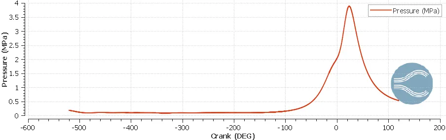

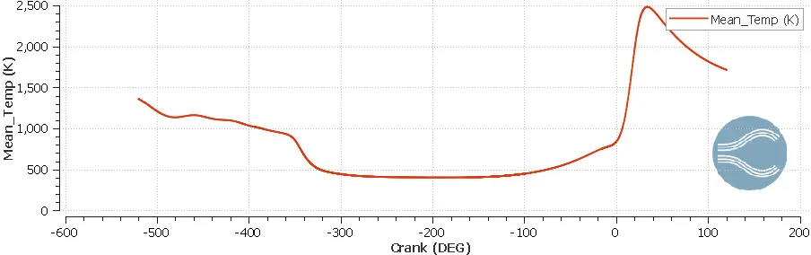
The mean temperature at the beginning is around 1400K which depicts the exhaust gases flowing out of the cylinder at that point. The temperature is at it’s the lowest point of 400K at -200 degrees crank angle showing the exhaust. It reaches its peak of 2500K at around 22 degrees indicating the point of combustion of the fuel.

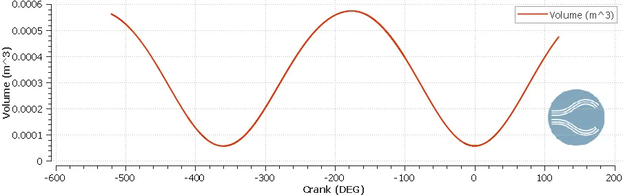
The total volume of the mixture trapped inside the cylinder at a particular crank angle is depicted in the figure. The wavy nature can be attributed to the different strokes of the combustion cycle. The ratio of max volume to minimum volume represents the compression ratio of the cylinder. In this case,

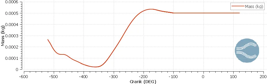
The total mass trapped inside the cylinder is provided in the figure below. The lowest mass trapped is 2e-5 kg at -350 degrees showing that most of the gas has been pushed out of the cylinder via the exhaust valve. At around -180 degrees, the inlet valve opens, and hence the mass trapped increases reaching a peak of 0.0053 kg.

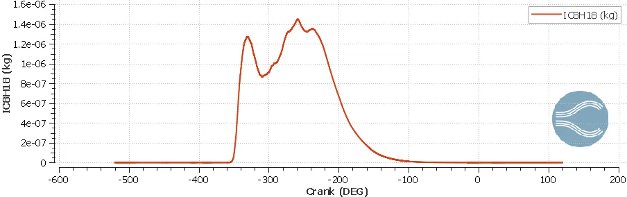
The heat release integrated over the cycle is provided in the figure below. This is an important factor that helps in determining the combustion efficiency of the cylinder. Combustion efficiency is the fraction of the fuel that burns.

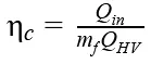
Where Qin=1.241kJ (from the graph)

QHV=44000 kJ/kg-k (standard value for gasoline)

mf=3e-5 kg (given data)

∴ ηc=0.94=94%

This implies that for every 100 liters of fuel put in, 94 liters get burned

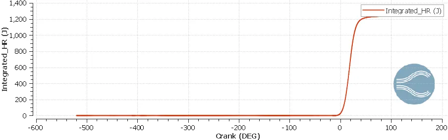
The next graph is the gamma value varying in accordance with the crank angle. The gamma value is generally taken to be 7/5 or 1.4 for diatomic gas during hand calculations but in actual simulation, the values vary in accordance with the crank angle. Hence simulations yield better results compared to other forms of arriving at conclusions.

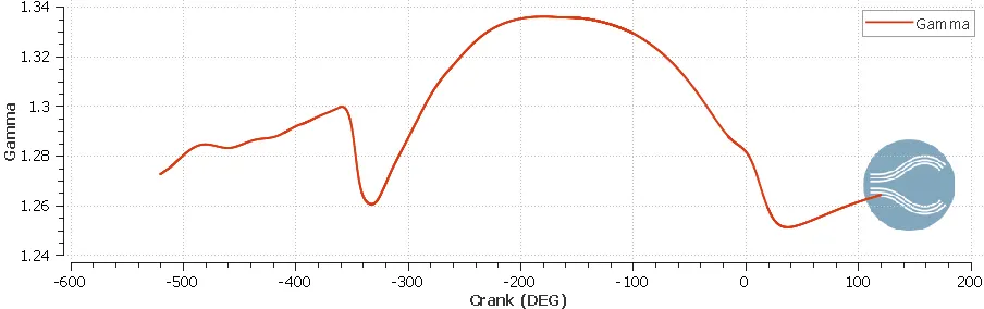
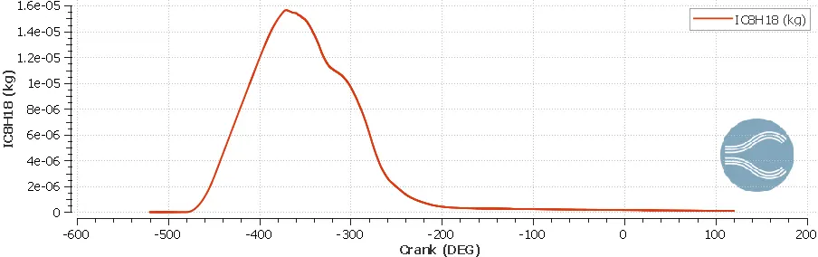
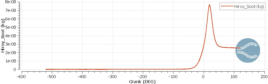
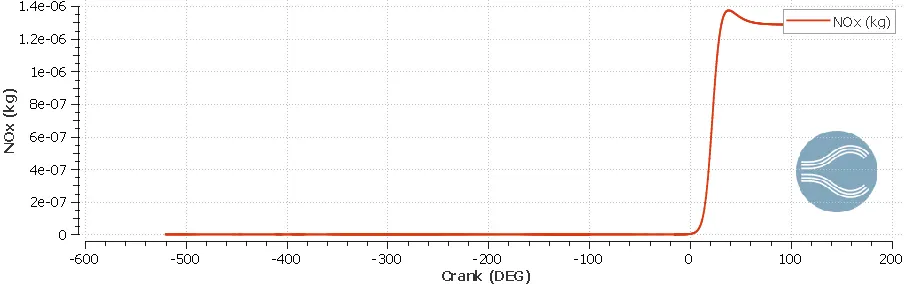
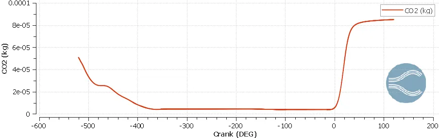
Another important set of values to look at are the emissions. The different compounds formed after combustion and its variation with the crank angle are provided in the following graphs. The products include CO2, NOx, and soot formation as seen below.

Engine performance:

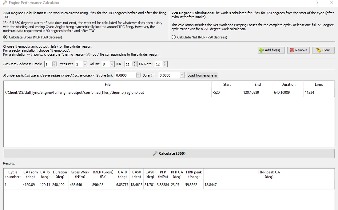
The Thermo file for the cylinder was input and the engine physical parameters were obtained by loading the engine.in file. The values that were obtained are shown below.

Engine performance:

The Thermo file for the cylinder was input and the engine physical parameters were obtained by loading the engine.in file. The values that were obtained are shown below.

The ca10 ca50 and ca90 are the crank angles at which the corresponding number percentages have been combusted. That is, a ca10 of 6.8 degrees imply that 10% of cmubstion is completed at a crank angle of 6.8 degrees and so on.

To get the values of power and torque, the following steps were taken:

Given, N=3000 rpm=50 revs/second

So since there are 360degrees in a rev, there would be 50*360=18000 degrees/ second and hence it takes 55μs to turn a degree. The power stroke is 240 degrees as seen in the screenshot below and hence, it would take 55μs*240=0.0133 seconds to turn through 240 degrees.

∴ Power= workdone/second= 468.646/0.0133=35.1kW

Power=2*3.14*N*T/60000 kW

Torque=111.78 N-m/rad

Conclusions:

The engine was setup in a detailed manner and results obtained were faithful. The link to the video would be https://youtu.be/Ti0Om4zfK8c