Week 7: Shock tube simulation project

AIM:
The simulation of the 3D Shock tube was performed using Converge 3.0, as part of this project.

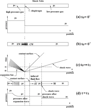
Shock tubes are utilized to replicate blast waves and simulate the effects of explosions on a smaller scale, as well as to examine compressible flow phenomena and gas-phase combustion reactions. A shock wave can be generated inside a shock tube by a small explosion (blast-driven) or by the buildup of high pressures causing diaphragm(s) to rupture and a shock wave to propagate down the shock tube (compressed-gas driven). When the diaphragm ruptures, a compression wave is created that propagates through the low-pressure section, along with expansion waves traversing the high-pressure section. After a short time, the compression waves merge to form the shock wave, which propagates through the low-pressure section. The stationary low-pressure gases experience a rise in pressure and temperature due to the arrival of shock waves, as shown in the figure below. The closed ends of the tube reflect both the expansion fan and shock waves. The reflected shock wave counters the motion of the low-pressure section initiated by the primary shock. The strength of the shock wave and expansion fan depends on the initial pressure ratio across the diaphragm and the physical properties of the gases in the sections.

PROCEDURE:

The workflow for the simulation in Converge is as follows:

1. Import the 3D geometry into the Converge workspace.
2. Assign appropriate names to the boundaries and check the normal directions to ensure they align with the geometry and flow.
3. Perform a diagnosis to identify any discrepancies in the geometry.
4. Select appropriate species for each region.
5. Set the simulation parameters, including appropriate time steps.
6. Define the boundary conditions and their corresponding values for each region.
7. Insert the base grid with the desired step size and appropriate AMR of 3 embedded layers with species SGS of 0.001.
8. Specify the variables for post-processing and the time intervals for writing the output and restart files.
9. Store all input files in the desired location.
10. Execute all stored input files using the command editor, which is run by the Converge Solver in the background.
11. The executed files generate an output folder where data files after every selected cycle interval are stored for post-processing and graphical results.

Geometry:

Box with below Dimensions:

• Length: 0.2m
• Breadth: 0.01m
• Height of 0.01m, is modeled with two regions as below.

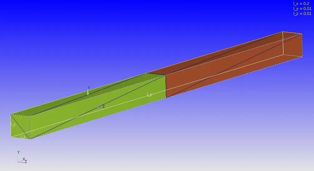
Green Region - High-Pressure Area (N2 gas)

Brown Region - Low-Pressure Area (O2 gas)

Both regions in the simulation are controlled by events, which act as a diaphragm to generate the shock and to separate the regions prior to the explosion (i.e., the diaphragm opening).

Case Setup:

Type of simulation: Transient Pressure-Based

Model: RNG k-ε

Materials: O2 & N2

Simulation Time: 0-0.003 s

Boundary Conditions:

• Walls (slip)
• High-Pressure Region (N2, 6e5 Pa, 300K)
• Low-Pressure Region (O2, 101325 Pa, 300K)

Events:

• Closed: 0 - 0.001s.
• Open: 0.001 - 0003s.

Adaptive Mesh Refinement:

• 0.001m Base Grid
• Refinement based on N2 species SGS: 0.001

Mesh:

A base grid size of 0.001m is implemented in all directions. The Adaptive Mesh Refinement (AMR) strategy uses a sub-grid scale criterion of 0.001 for 3 embedded layers, specifically for the N2 species.

AMR is activated if the below criterion is met.

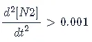
When the AMR sub-grid scale criterion is satisfied, the size of the three embedded layers adjacent to the cell is halved without any scaling.

Mesh refinement during simulation is shown in below video:

Grid Dependency Test:

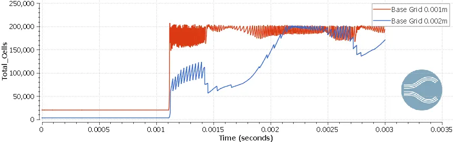
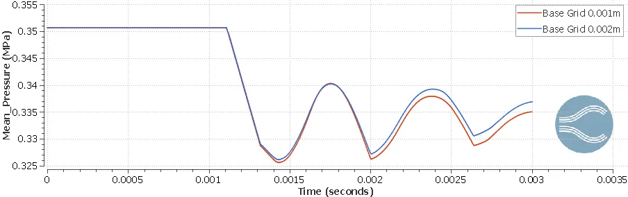
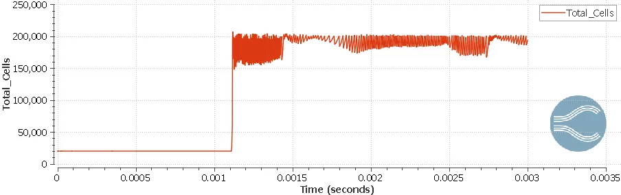
For the grid dependency study, two base grid sizes, 0.002m and 0.001m, are analyzed. The total number of cells, as well as the variation of mean pressure and temperature in both regions over the simulation time, are compared for both grid sizes.

Total Cells:

Variation of Pressure in the flow region:

Variation of Temperature in the flow region:

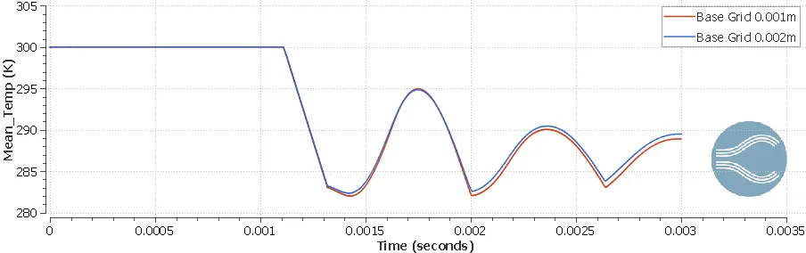
The results in the above figures indicate that the differences between the 0.002m and 0.001m base grid sizes are within 1%. The number of cells in the simulation with a 0.001m base grid is significantly higher. Therefore, a base grid size of 0.002m is preferred. However, for this project, a base grid size of 0.001m was chosen.

Total Cells:

The total number of cells over the simulation time is illustrated below:

Effect on Mass Fraction and Pressure:

Effect on Mass Fraction and Velocity:

Variation of Temperature in Shock Tube:

Variation of Density in Shock Tube:

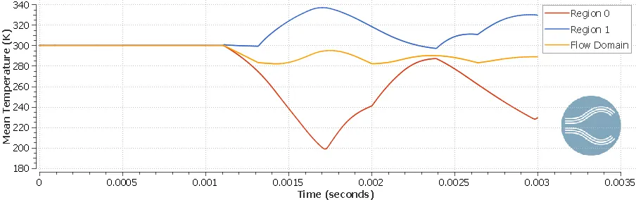
Mean Temperature over Flow Time:

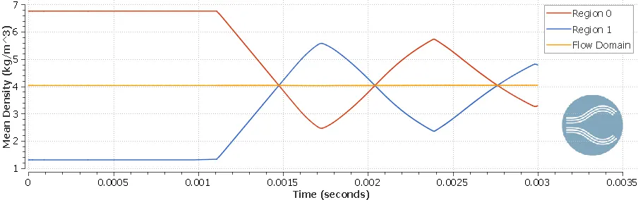
Mean Density over Flow Time:

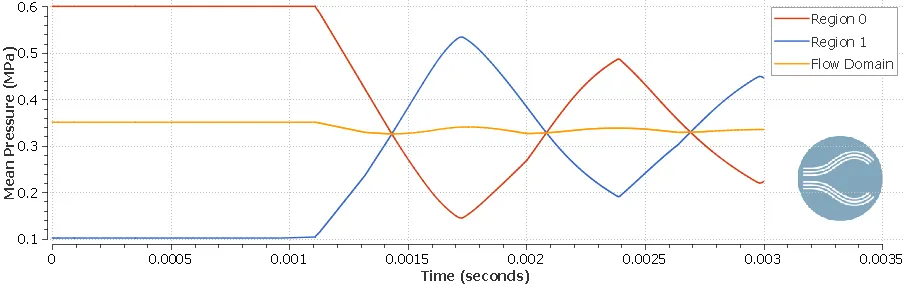
Mean Pressure over Flow Time:

CONCLUSION

• The process of generating shock and expansion waves continues until the pressure difference in the domain diminishes, and AMR keeps refining the mesh in the wavefront until the rate of change of N2 concentration falls below the SGS value.
• To observe the pressure difference damping, the simulation needs to run for a longer duration.
• At 0.001s, the diaphragm breaks (activated by events), and the pressure in the High-pressure region decreases, causing an increase in the Low-pressure region's pressure, leading to a shock in the Low-pressure region and corresponding expansion waves due to the pressure decrease, flowing in the High-pressure region.
• The shock waves reflect when the gases in the Low-pressure region are compressed, and the pressure in the Low-pressure region is higher than the Shock front.
• This sinusoidal behavior of damping is observed until the pressure difference becomes zero.
• The density variation follows the same pattern as the pressure because both of them are directly related to the ideal gas equation.
• Additionally, the shock increases the temperature, and the expansion wave decreases it.