Week 6: Conjugate Heat Transfer Simulation

AIM:

The aim of this study is to simulate the flow of fluid through a heated, hollow aluminum cylinder, investigate the conjugate heat transfer, and perform a grid dependence test. Additionally, the effect of the super-cycling stage interval on simulation results will also be examined.

PROCEDURE:

• The simulation process began by creating the geometry in Converge Studio and performing a thorough error check. The geometry was then grouped into faces, and the appropriate boundary conditions were assigned.

• This is a transient simulation with a duration of 0.5 seconds, using the RNG k-epsilon turbulence model since it is a turbulent flow simulation. Mesh sizes of 2e-3m, 3e-3m, and 4e-3m were utilized in all directions.

• The Navier-Stokes Unsteady equations were used to solve this case, which included five equations: the continuity equation, the x-momentum equation, the y-momentum equation, the z-momentum equation, and the energy equation.

• A super-cycling stage interval of 0.05s was employed in this project. In the super-cycling method, the fluid solver is temporarily paused to allow the solid solver to catch up

GEOMETRY:

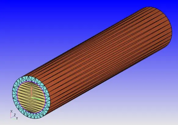
Cylinder Dimensions:

• Length: 0.2m
• Inner Diameter: 0.015m
• Outer Diameter: 0.02m

Material:

• Fluid: Air
• Solid: Aluminium

Boundary Condition:

• Inlet: Velocity: 7.32m/s
• Outlet: Pressure 101325 Pa
• Solid outer wall: 10000 W/m2
• Solid wall: No Slip - Fixed wall.
• Interface: Fluid region - Forward boundary & Solid region - Reverse boundary

Initial Parameters:

• Pressure: 101325 Pa
• Temperature: 300K

MESH:

1. 2e-3m

2. 3e-3m

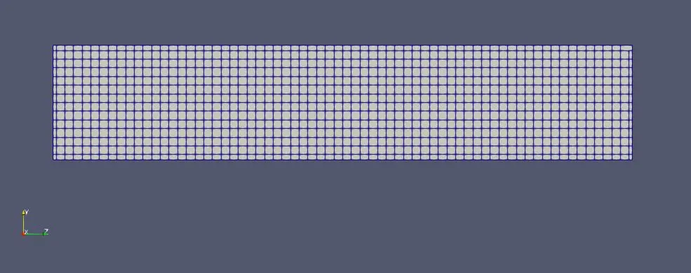
3. 4e-3m

RESULTS:

Cell-Count

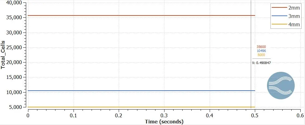
Thus, from the above Line plot, we can conclude saying that, it's clear that Mesh size & Cell Count are inversely proportional where as the mesh size decreases the cell count increases.

For Case 1 - Mesh: 2e-3m:

Pressure:

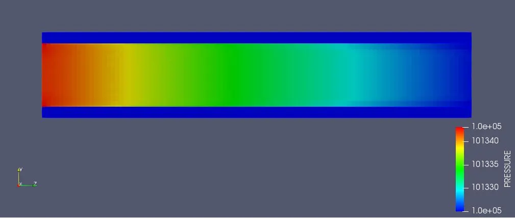
Based on the pressure plot analysis, it can be observed that the flow is taking place from the inlet to the outlet without any reverse flow

Temperature:

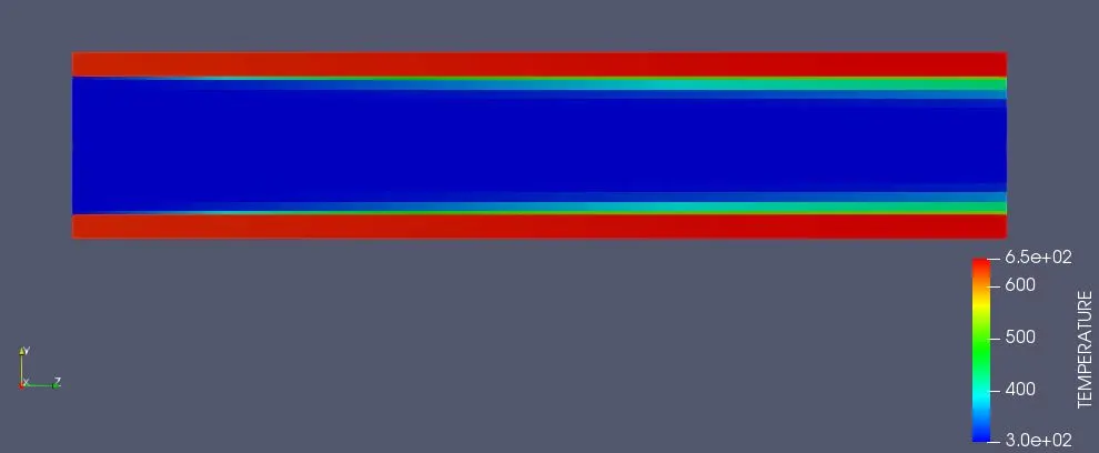
According to the temperature plot analysis, it is evident that the temperature of the air increases as it moves toward the outlet, which is consistent with the average temperature line plot.

Velocity:

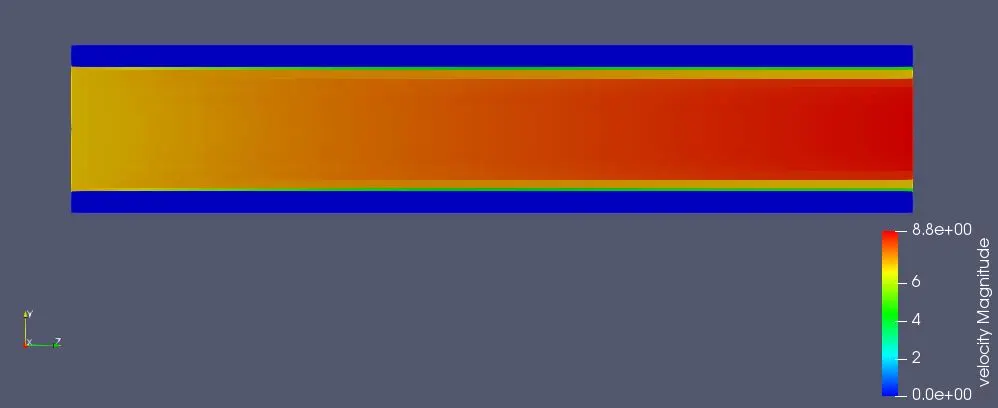
Based on the velocity plot analysis, it can be observed that the velocity of the air increases as it flows from the inlet to the outlet. This phenomenon can be attributed to the increase in temperature along the pipe.

Y+:

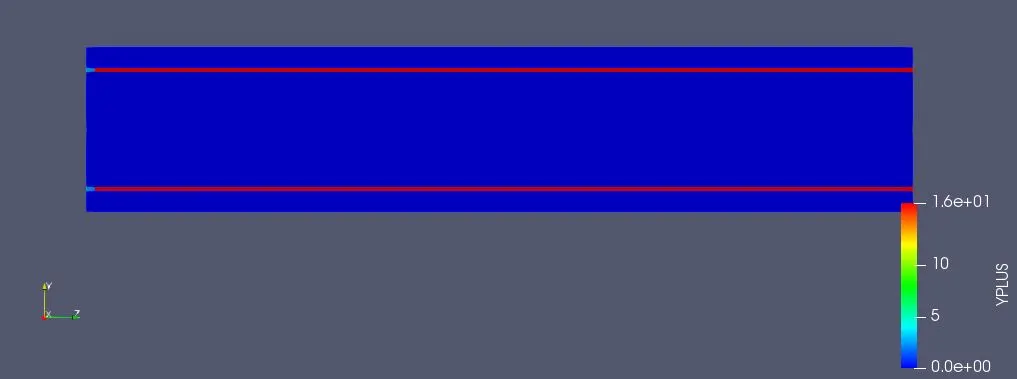
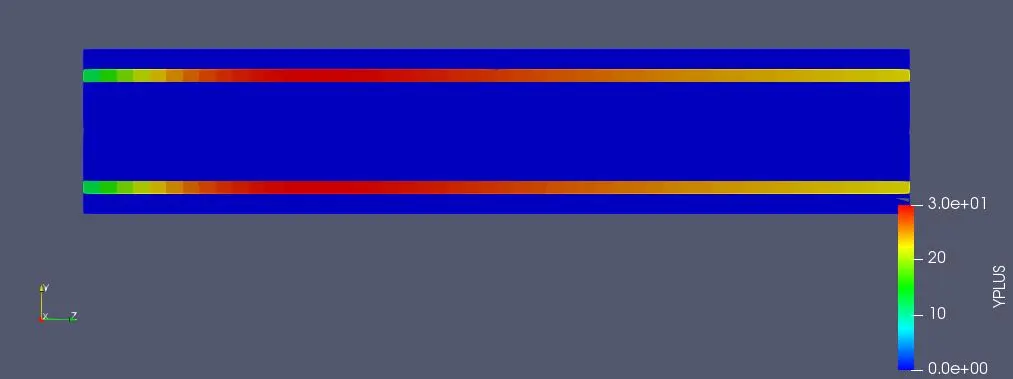
Thus, as the mesh gets fine, y+ decreases.

For Case 2 - Mesh: 3e-3m:

Pressure:

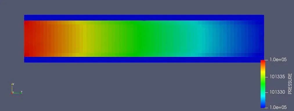
According to the pressure plot analysis, it can be concluded that the flow direction is from the inlet to the outlet, i.e., from left to right. Moreover, there is no indication of any reverse flow occurring in the system.

Temperature:

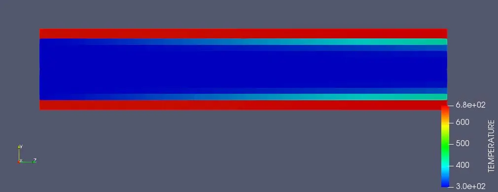
The temperature plot verifies the average temperature line plot, indicating that the temperature of the air rises as it moves closer to the outlet.

Velocity:

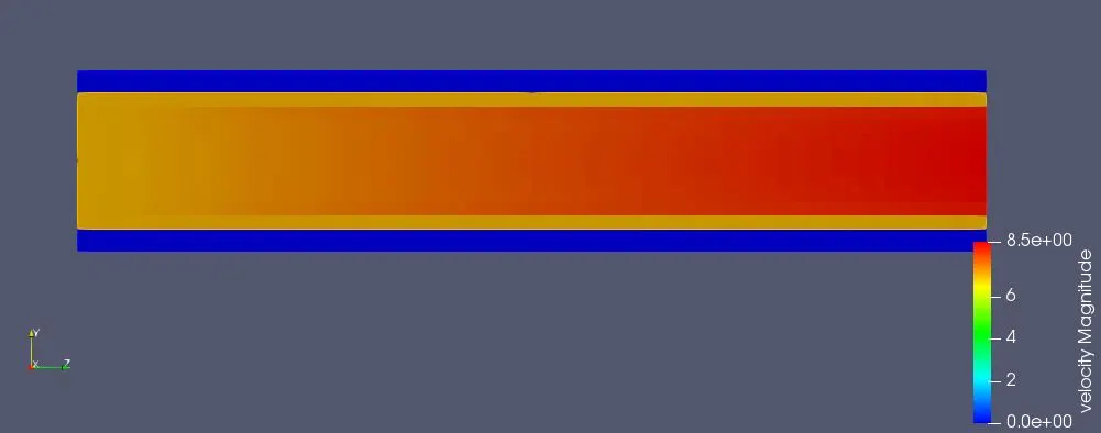
The velocity plot shows an increase in velocity from the inlet to the outlet, which can be attributed to the decrease in cross-sectional area of the pipe. This is due to the continuity equation, which states that the product of velocity and cross-sectional area is constant in an incompressible fluid. Therefore, as the cross-sectional area decreases towards the outlet, the velocity increases to maintain a constant mass flow rate.

Y+:

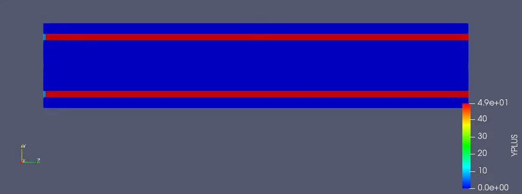
For Case 2 - Mesh: e-3m:

Pressure:

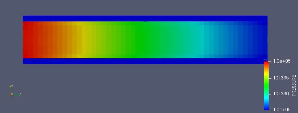
From the pressure plot, it is clear that the flow is taking place from left to right i.e inlet to outlet and no reverse flow is occurring.

Temperature:

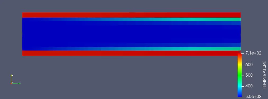
The temperature distribution along the pipe can be observed from the temperature plot. It shows that the temperature of air increases gradually as it moves towards the outlet. This is consistent with the expected behavior of the heated cylindrical pipe.

Velocity:

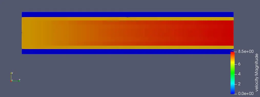
From the above velocity plot, it indicates that the velocity profile is positively correlated with the temperature profile, with the velocity increasing as the temperature increases along the pipe from the inlet to the outlet.

Y+:

CONCLUSION:

• The temperature profiles at the outlet show similar results, indicating that the solution is not grid-dependent.
• To analyze the impact of different super-cycling stage intervals on the simulation time, three simulations were conducted using intervals of 0.01s, 0.02s, and 0.03s.
• The simulation time for the 0.01s super-cycling interval was 597.19 seconds.
• The simulation time for the 0.02s interval, it was 593.36 seconds.
• The simulation time for the 0.03s interval, it was 591.35 seconds.
• The trend indicates that an increase in the super-cycling interval leads to a decrease in simulation time.