Week 7: Shock tube simulation project
Hello,
In this shoch tube challenge, as per the given problem statements, first we find the respective parameters to set our case setup accordingly and plan the simulation. To do the same, first go for importing the geometry in the CONVERGE-STUDIO. After this, go for the normal checks, which must be pointed in the direction of the flow. Then, a diagnosis is done to check for any kind of geometrical error. After verifying it, the case setup is set as per the given inputs and boundary conditions. In this case, all the basic parameters are selected with specific values, and all these values are setup together as input files for the model. During the case setup, the important thing that we need to keep in mind is that the there are 2 regions are there i.e. high and low pressure region having N2 and O2 gas respectively at 6bar and 1 bar pressure. Hence there are tw regions one event is imortant to be created in between them that opens after 0.001 sec. Then after completing the case setup, we need to export the files.
The simulation that follows can be converging by using the Cygwin interface, which is required for giving the command to the software. In Cygwin, first we go to the directory where the input files are present and then command them for simulation. This simulation can be done automatically at the back end, and the output files are generated in the same folder as the results of the simulation.
Then those output files have to be exported in Paraview to see the results in the different interfaces and also in their plots in the Converge Studio. For importing the output files in Paraview, first we need to convert the data into a ".vtm file," which is done in the "Post-Processing 3-D" option in Converge-Studio. Then all the 3D and 2-D analyses of the results are analysed separately. The rest of the plots can be seen in Converge-studio itself, specifically under the "line-plotting option."
By doing so, I was able to obtain all of the required results for this particular challenge and take screenshots of them. The CFD analysis of this problem is done three times for three different mesh sizes, and the results are attached in a word file. Kindly find it below.
Detailed explanations about the plots:
Cell count: The cell count in this challenge is constant from the beginning to the end because there is no adaptive mesh refinement that we are using that would fluctuate the number of cells throughout the simulation process. But as we see the overall after 0.001sec as the event opens the cell count increased in a fluctuating manner due to species AMR.
The mass flow rate plots appear to be unstable at first touch, but as the flow cycled on, convergence took effect. After achieving the convergence shown in the graph, we observe that the mass of the flow that enters the geometry from the inlet per unit of time is equal to the mass of the flow that exits from the outlet. But due to the sign conventions, the input and output flows are represented, respectively, as positive and negative values for comparison.
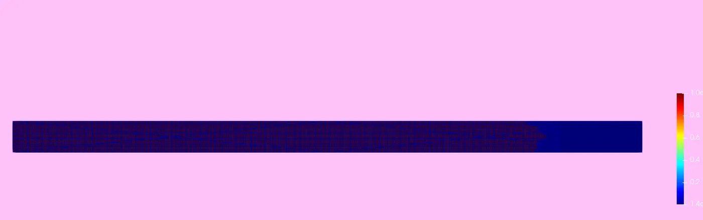
Mesh with dx=dy=dz=0.004 m is been set in the model with AMR on species i.e. on N2 mass fraction
Pressure: As soon as the event breaks apart, a shock pulse is generated. The sudden drop in pressure on the high-pressure side is what causes a shock wave to be created. The back pressure created by the reflected waves causes the low-pressure side to experience a rise in pressure, which then spreads to cover the high-pressure side. In the results, also parallel pressure fluctuation between areas is observed.
Temprature: The curve of temperature also exhibits the same pattern as that of pressure. The temperature immediately drops in the N2 region. The backpressure created by reflected waves raises the temperature on the O2 side, which then blankets the high pressure side. Both results are attached to the word file below.