Aerofoil Simulation

NACA 0012 AIRFOIL

The NACA airfoils are airfoil shapes for aircraft wings developed by the National Advisory Committee for Aeronautics (NACA). The shape of the NACA airfoils is described using a series of digits following the word "NACA". The parameters in the numerical code can be entered into equations to precisely generate the cross-section of the airfoil and calculate its properties.

NACA initially developed the numbered airfoil system,, further refined by the United States Air Force at Langley Research Center. According to the NASA website:

During the late 1920s and into the 1930s, the NACA developed a series of thoroughly tested airfoils and devised a numerical designation for each airfoil — a four-digit number representing the airfoil section's critical geometric properties. By 1929, Langley had developed this system to the point where the numbering system was complemented by an airfoil cross-section, and the complete catalog of 78 airfoils appeared in the NACA's annual report for 1933. Engineers could quickly see the peculiarities of each airfoil shape, and the numerical designator ("NACA 2415," for instance) specified camber lines, maximum thickness, and special nose features. These figures and shapes transmitted the sort of information to engineers that allowed them to select specific airfoils for desired performance characteristics of specific aircraft.

The NACA four-digit wing sections define the profile by:

1. First digit describing maximum camber as a percentage of the chord.
2. The second digit describing the distance of maximum camber from the airfoil leading edge in tenths of the chord.
3. Last two digits describing the maximum thickness of the airfoil as the percent of the chord.

For example, the NACA 2412 airfoil has a maximum camber of 2% located 40% (0.4 chords) from the leading edge with a maximum thickness of 12% of the chord.

The NACA 0015 airfoil is symmetrical, the 00 indicating that it has no camber. The 15 indicates that the airfoil has a 15% thickness to chord length ratio: it is 15% as thick as it is long.

The equation for a symmetrical 4-digit NACA airfoil

The formula for the shape of a NACA 00xx foil, with "xx" being replaced by the percentage of thickness to chord, is

where:

x is the position along the chord from 0 to 1.00 (0 to 100%),

is the half-thickness at a given value of x (centerline to the surface),

t is the maximum thickness as a fraction of the chord (so t gives the last two digits in the NACA 4-digit denomination divided by 100).

Note that the thickness is not quite zero in this equation at x = 1 (the trailing edge of the airfoil). If a zero-thickness trailing edge is required, for example for computational work, one of the coefficients should be modified such that they sum to zero. Modifying the last coefficient (i.e. to −0.1036) will result in the smallest change to the overall shape of the airfoil. The leading edge approximates a cylinder with a chord-normalized radius of

Now the coordinates of the upper airfoil surface and of the lower airfoil surface are

Symmetrical 4-digit series airfoils by default have a maximum thickness at 30% of the chord from the leading edge.

The equation for a cambered 4-digit NACA airfoil

The simplest asymmetric foils are the NACA 4-digit series foils, which use the same formula as that used to generate the 00xx symmetric foils, but with the line of mean camber bent. The formula used to calculate the mean camber line is

where

m is the maximum camber (100 m is the first of the four digits),

p is the location of the maximum camber (10 p is the second digit in the NACA XXXX description).

For example, a NACA 2412 airfoil uses a 2% camber (first digit) 40% (second digit) along the chord of a 0012 symmetrical airfoil having a thickness of 12% (digits 3 and 4) of the chord.

For this cambered airfoil, because the thickness needs to be applied perpendicular to the camber line, the coordinates and, of respectively the upper and lower airfoil surface, become

where

SIMULATION CASE 1[ANGLE OF ATTACK = 5 DEG]

Mesh

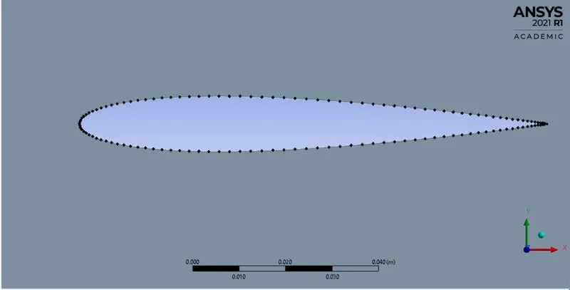
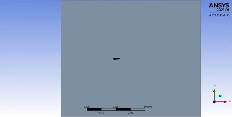
Steps to create the geometry shape of the NACA 0012 airfoil.

1. Create the points necessary for the airfoil.
2. Next, we join the points to form a line and create the surface of the airfoil
3. Then according to the dimensions, we have to form the bounding box or enclosure.
4. Then we subtract the airfoil surface by boolean operation.

Mesh

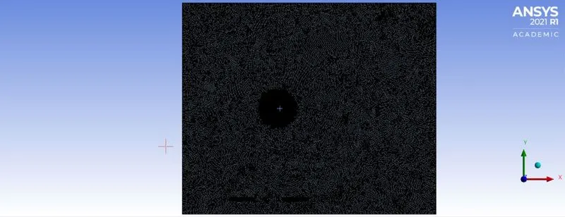
Now in the mesh is created using body sizing and edge sizing methods. The base size of 10mm with the mesh size of 3mm in body sizing takes the count of elements to 255232.

Body Sizing allows you to add sizing to an entire selected body or body. This will essentially overwrite the global controls specified and useful when you have multiple bodies and need to control the sizing in certain bodies individually. This may be the case if you need different quality meshes in solid and fluid components for a conjugate heat transfer problem, where you will need to accurately resolve the flow and thermal boundary layer in the fluid domain (which are essential to accurate calculations of the heat transfer), but can afford to tolerate a lower fidelity mesh in the solid components. The Body Sizing function also has the option to set a growth rate. This will use the global values by default, but we can also define a local value that overrides the global settings and gives us individual control over the mesh for multiple bodies.

1. Geometry - Body selected
2. Type - Sphere of Influence
3. Sphere Center - Global co-ordinate systems
4. Sphere Radius - 150mm
5. Element Size - 3mm

Edge Sizing Controls can be given to any edge and allow for different types of bias control, whereby the mesh size varies along the edge. In the image below, we have applied edge sizing to a single edge.

The edge sizing feature can use either a specified element size, several divisions along the edge, or controlled by a sphere of influence. This last option will refine along the edge only where it is intersected by the sphere of influence, and we will show this later on in this blog post.

Within the edge sizing function, you have the ability to set a local growth rate for all cells that grow away from this edge (overriding the global growth rate). There are also useful options for Edge Bias control, which allows you to define how the mesh is distributed along the length of the edge. For example, you can force the mesh along the edge to vary from large to small, small to large; or more complicated bias such as large to small in the middle then back to large, or small to large in the middle, and then back to small again at the other end of the edge.

1. Geometry - edge selection
2. Behavior - Hard
3. Bias type - Dash line
4. Bias Factor - 10

Setup

The simulation steps were set up as follows

1. Solver - Pressure
2. State - Steady state
3. Turbulence Model - K-Omega SST
4. Material - Air
5. Density = 2.131 kg/m^3
6. Angle of attack = 5 Degrees
7. Boundary Conditions

Inlet

1. Inlet - Velocity Inlet
2. Velocity - Components
3. X velocity = 51.802 m/s
4. Y velocity = 4.53 m/s
5. Temperature = 300 K

Outlet

1. Pressure Outlet
2. Pressure = 0 Pa

Wall

1. Wall Boundary
2. No Slip BC

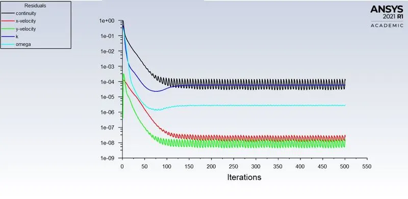
Residual Plot

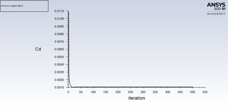
Coefficient of Drag

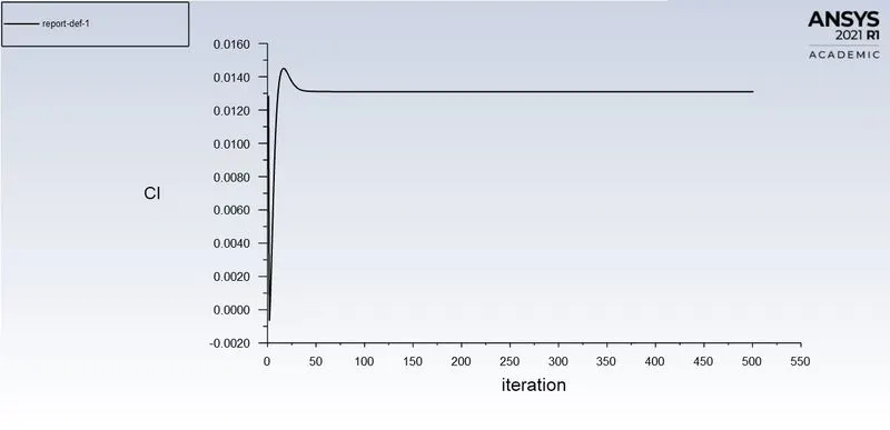
Coefficient of Lift

Results

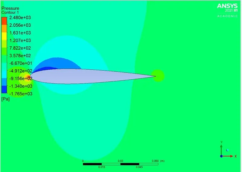
Pressure Countour

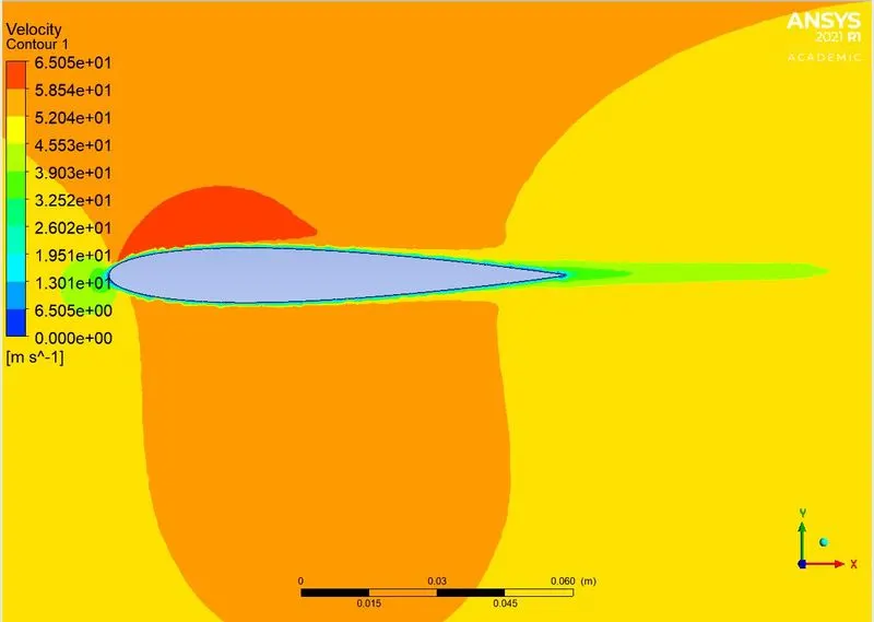
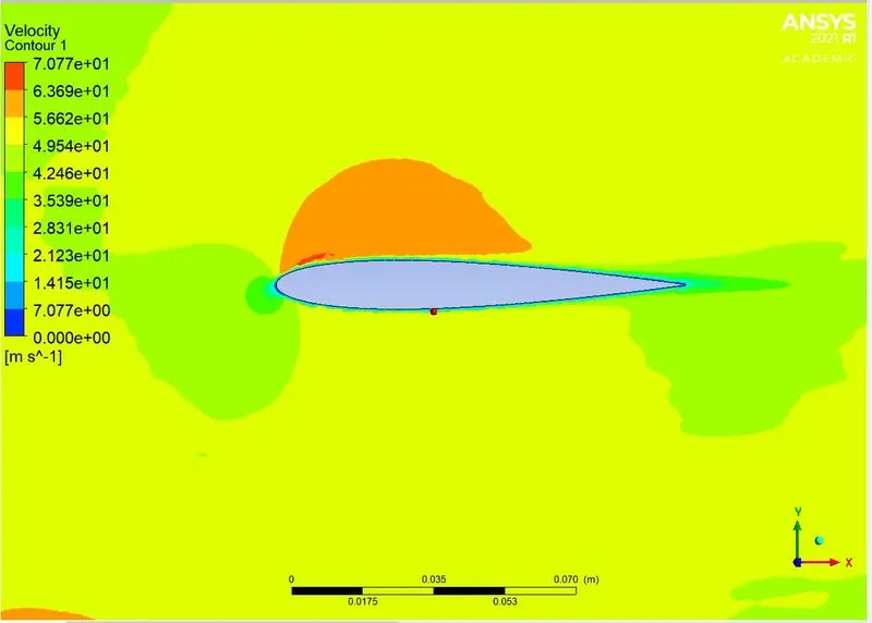
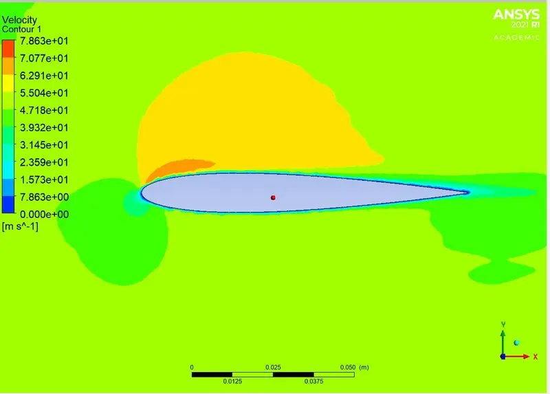
Velocity Contour

SIMULATION CASE 1[ANGLE OF ATTACK = 10 DEG]

Mesh

Steps to create the geometry shape of the NACA 0012 airfoil.

1. Create the points necessary for the airfoil.
2. Next, we join the points to form a line and create the surface of the airfoil
3. Then according to the dimensions, we have to form the bounding box or enclosure.
4. Then we subtract the airfoil surface by boolean operation.

Mesh

Now in the mesh is created using body sizing and edge sizing methods. The base size of 10mm with the mesh size of 3mm in body sizing takes the count of elements to 255232.

Body Sizing allows you to add sizing to an entire selected body or body. This will essentially overwrite the global controls specified and useful when you have multiple bodies and need to control the sizing in certain bodies individually. This may be the case if you need different quality meshes in solid and fluid components for a conjugate heat transfer problem, where you will need to accurately resolve the flow and thermal boundary layer in the fluid domain (which are essential to accurate calculations of the heat transfer), but can afford to tolerate a lower fidelity mesh in the solid components. The Body Sizing function also has the option to set a growth rate. This will use the global values by default, but we can also define a local value that overrides the global settings and gives us individual control over the mesh for multiple bodies.

1. Geometry - Body selected
2. Type - Sphere of Influence
3. Sphere Center - Global co-ordinate systems
4. Sphere Radius - 150mm
5. Element Size - 3mm

Edge Sizing Controls can be given to any edge and allow for different types of bias control, whereby the mesh size varies along the edge. In the image below, we have applied edge sizing to a single edge.

The edge sizing feature can use either a specified element size, several divisions along the edge, or controlled by a sphere of influence. This last option will refine along the edge only where it is intersected by the sphere of influence, and we will show this later on in this blog post.

Within the edge sizing function, you have the ability to set a local growth rate for all cells that grow away from this edge (overriding the global growth rate). There are also useful options for Edge Bias control, which allows you to define how the mesh is distributed along the length of the edge. For example, you can force the mesh along the edge to vary from large to small, small to large; or more complicated bias such as large to small in the middle then back to large, or small to large in the middle, and then back to small again at the other end of the edge.

1. Geometry - edge selection
2. Behavior - Hard
3. Bias type - Dash line
4. Bias Factor - 10

Setup

The simulation steps were set up as follows

1. Solver - Pressure
2. State - Steady state
3. Turbulence Model - K-Omega SST
4. Material - Air
5. Density = 2.131 kg/m^3
6. Angle of attack = 10 Degrees
7. Boundary Conditions

Inlet

1. Inlet - Velocity Inlet
2. Velocity - Components
3. X velocity = 51.21 m/s
4. Y velocity = 9.029 m/s
5. Temperature = 300 K

Outlet

1. Pressure Outlet
2. Pressure = 0 Pa

Wall

1. Wall Boundary
2. No Slip BC

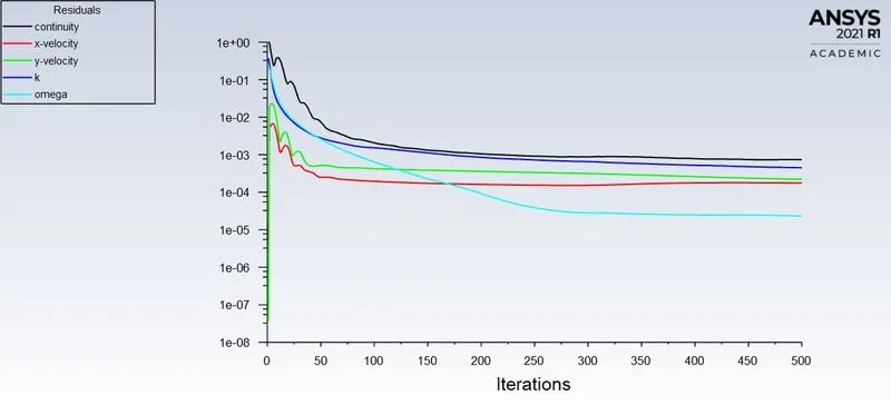
Residual Plot

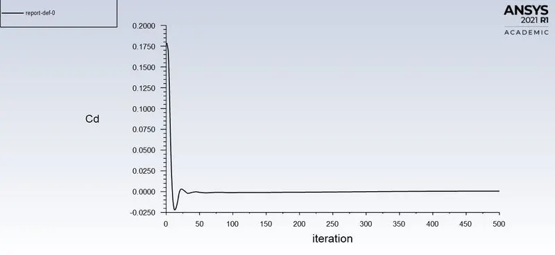
Coefficient of Drag

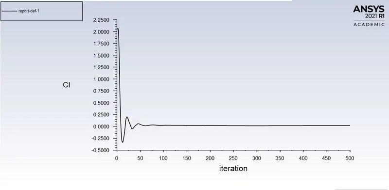
Coefficient of Lift

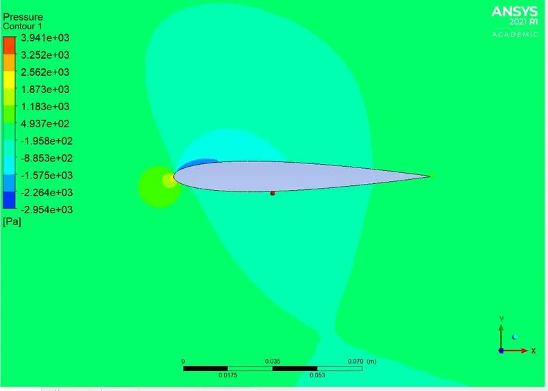
Results

Pressure Contour

Velocity Contour

SIMULATION CASE 1[ANGLE OF ATTACK = 15 DEG]

Mesh

Steps to create the geometry shape of the NACA 0012 airfoil.

1. Create the points necessary for the airfoil.
2. Next, we join the points to form a line and create the surface of the airfoil
3. Then according to the dimensions, we have to form the bounding box or enclosure.
4. Then we subtract the airfoil surface by boolean operation.

Mesh

Now in the mesh is created using body sizing and edge sizing methods. The base size of 10mm with the mesh size of 3mm in body sizing takes the count of elements to 255232.

Body Sizing allows you to add sizing to an entire selected body or body. This will essentially overwrite the global controls specified and useful when you have multiple bodies and need to control the sizing in certain bodies individually. This may be the case if you need different quality meshes in solid and fluid components for a conjugate heat transfer problem, where you will need to accurately resolve the flow and thermal boundary layer in the fluid domain (which are essential to accurate calculations of the heat transfer), but can afford to tolerate a lower fidelity mesh in the solid components. The Body Sizing function also has the option to set a growth rate. This will use the global values by default, but we can also define a local value that overrides the global settings and gives us individual control over the mesh for multiple bodies.

1. Geometry - Body selected
2. Type - Sphere of Influence
3. Sphere Center - Global co-ordinate systems
4. Sphere Radius - 150mm
5. Element Size - 3mm

Edge Sizing Controls can be given to any edge and allow for different types of bias control, whereby the mesh size varies along the edge. In the image below, we have applied edge sizing to a single edge.

The edge sizing feature can use either a specified element size, several divisions along the edge, or controlled by a sphere of influence. This last option will refine along the edge only where it is intersected by the sphere of influence, and we will show this later on in this blog post.

Within the edge sizing function, you have the ability to set a local growth rate for all cells that grow away from this edge (overriding the global growth rate). There are also useful options for Edge Bias control, which allows you to define how the mesh is distributed along the length of the edge. For example, you can force the mesh along the edge to vary from large to small, small to large; or more complicated bias such as large to small in the middle then back to large, or small to large in the middle, and then back to small again at the other end of the edge.

1. Geometry - edge selection
2. Behavior - Hard
3. Bias type - Dash line
4. Bias Factor - 10

Setup

The simulation steps were set up as follows

1. Solver - Pressure
2. State - Steady state
3. Turbulence Model - K-Omega SST
4. Material - Air
5. Density = 2.131 kg/m^3
6. Angle of attack = 15 Degrees
7. Boundary Conditions

Inlet

1. Inlet - Velocity Inlet
2. Velocity - Components
3. X velocity = 50.22 m/s
4. Y velocity = 13.45 m/s
5. Temperature = 300 K

Outlet

1. Pressure Outlet
2. Pressure = 0 Pa

Wall

1. Wall Boundary
2. No Slip BC

Residual Plot

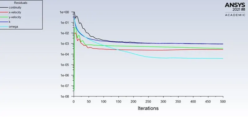
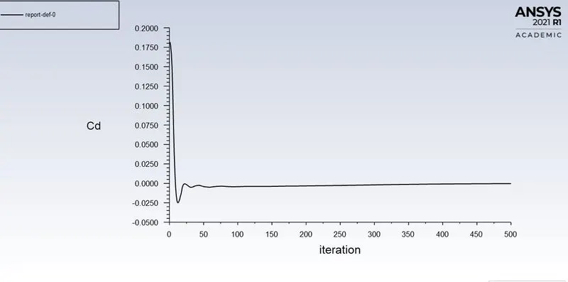
Coefficient of Drag

Coefficient of Lift

Results

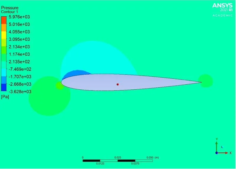
Pressure Contour

Velocity Contour

Case	Angle of attack	Coefficient of Drag	Coefficient of lift
1	5	0.00105	0.01309
2	10	0.00062	0.01657
3	15	0.00033	0.024806

CONCLUSION

1. The simulation was carried out with various angles of attack
2. As the angle of attack increases, the coefficient of drag is decreasing.
3. As the angle of attack increases, the coefficient of drag is also increasing