Week-7 : Converting a detailed engine model to a FRM model

• Explore tutorial number 9 and write a detailed report

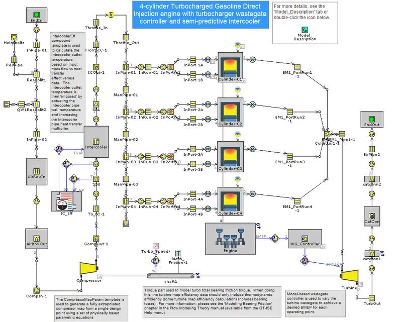
The model is a 4-cylinder 2.0 liter turbocharged Gasoline Direct Injection (GDI) engine as showm below.

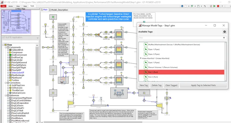
The 'FRM tags' option in the 'Tools' section shows the FRM tags which are already applied to the model. As shoem in the figure, it highlights the selected tagged part.

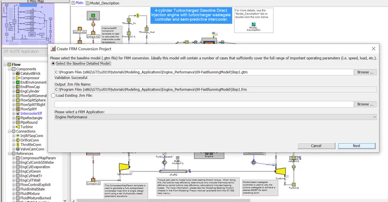
To convert the model to FRM, open 'FRM converter' in the 'Tools' section. It opens a new window where, the validation of the current model with existing FRM tags will carry out. Once the model is validated, confirm that the correct model is specified in "Select the Baseline Detailed Model" as shown below.

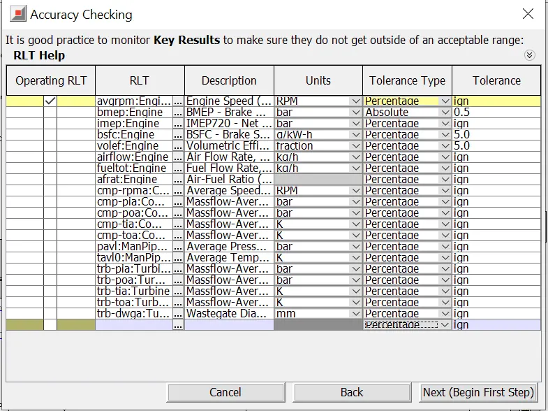
Once the validation is successfull, an "Accuracy Checking" dialog will appear to specify any optional tolerances.

After finalizing the "Accuracy Checking", atep 1 of conversion process will begin.

Step 1:

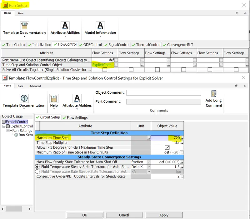
Before proceeding further, the maximum timestep in Run Setup is set to 720, inorder to make the timestep flexible according to the gas velocity and the length of the flow component.

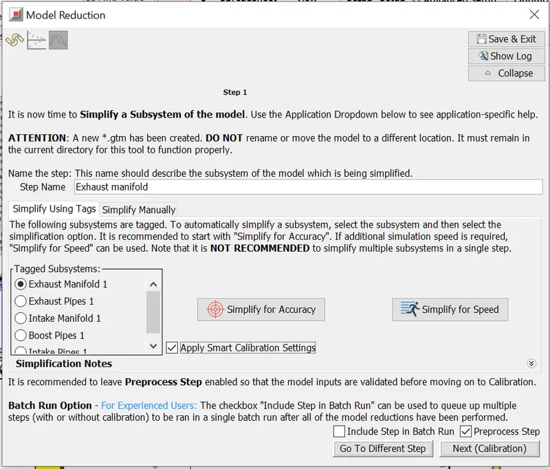
Once the model reduction page appears for step 1, inorder to start simplyfying the model, initially, the exhaust manifold, where the highest gas velocities occur, is selected. The "Apply Smart Calibration Settings" check box ahould be selected to prefills the attributes for the design optimizer
used later for model calibration steps. Also, "Simplify for Accuracy" or "Simplify for Speed" options can be selected depending on whether the point of interest is accuracy or speed. "Simplify for Accuracy" combines the valves, ports and runners of the exhaust valve.

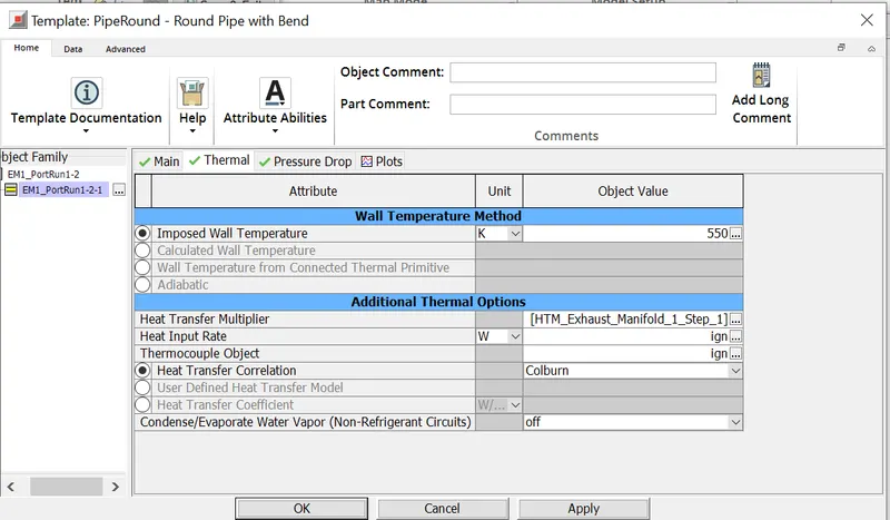
Once "Simplify for Accuracy" is clicked, it creates a heat transfer multiplier called [HTM_Exhaust_Manifold_1_Step_1] in the thermal tab of all port/runner pipes. It can be seen in the case setup and it changes according to the turbine inlet temperature.

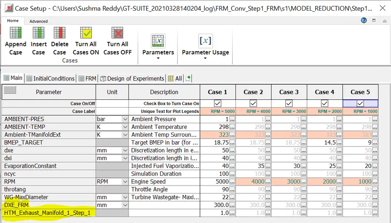
The case setup for newly created parameters is as follows.

After clicking "Next(Calibration)" in the "Model reduction" page, the model will preprocess and a calibration window opens. Here only case with high speed (5000 rpm) is selected as a first step as extra accuracy is not required in our case.

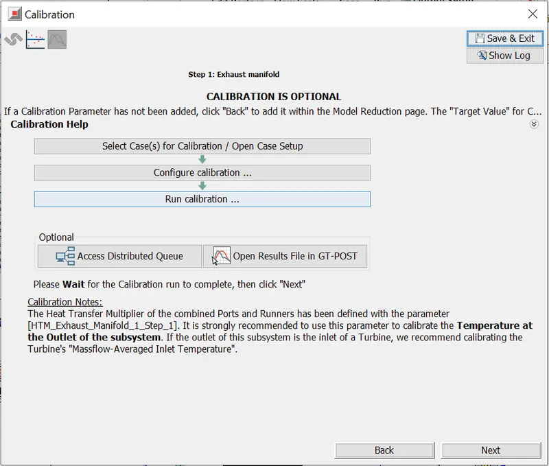
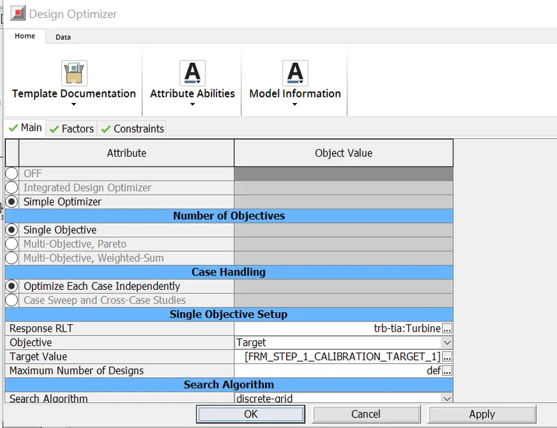
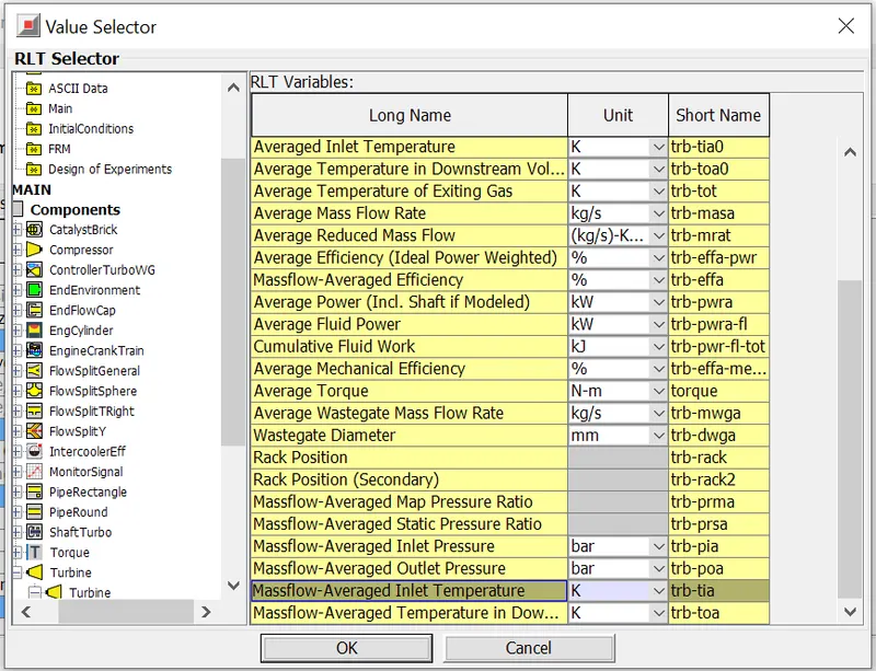
In the next step of "configure calibration" will open a design optimizer window. Here, in the "Response RLT", the option named, "Massflow Averaged Inlet Temperature" from the Turbine is selected.

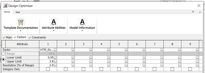
In the "factor" section of the "design optimizer" tab, the upper and lower limit of the ranges acn be selected.

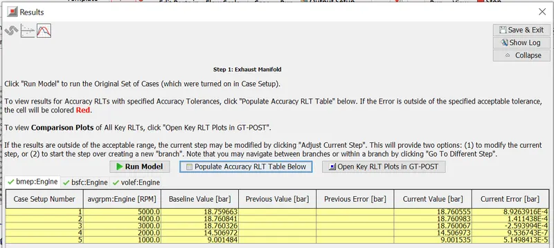
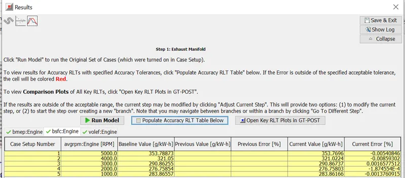
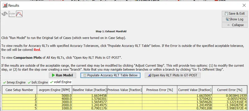
After selected the required parameters and values for the calibration, run the calibration. Once the simulation is finished, "Results" window will appear and by now all the cases in the case set up are turned on and the optimized parameter is applied to the model. Now, click "Run Model" to run all the cases with optimized parameter values. Once the model is simulated for all the cases, the results are as follows:

BMEP

BSFC

VOLUMETRIC EFFICIENCY

Step 2:

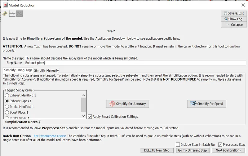
Now, we can proceed to next step. Here we select Exhaust pipes and click simplify for accuracy and move to Next (calibration).

In the model, select "EP1_Pipe1-1", "EP1_PDrop1-1" and the OrificeConn between them, then right click on the selection and launch the Combine Flow Volumes Wizard. Now select "Combine flow volumes to Flowsplit"

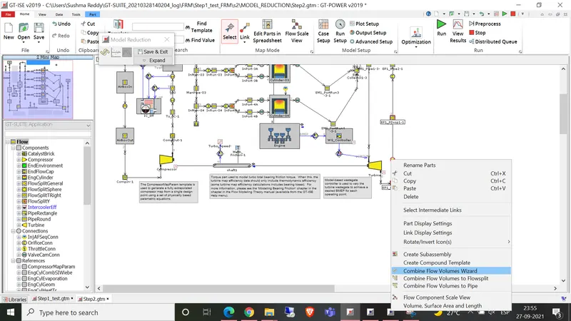
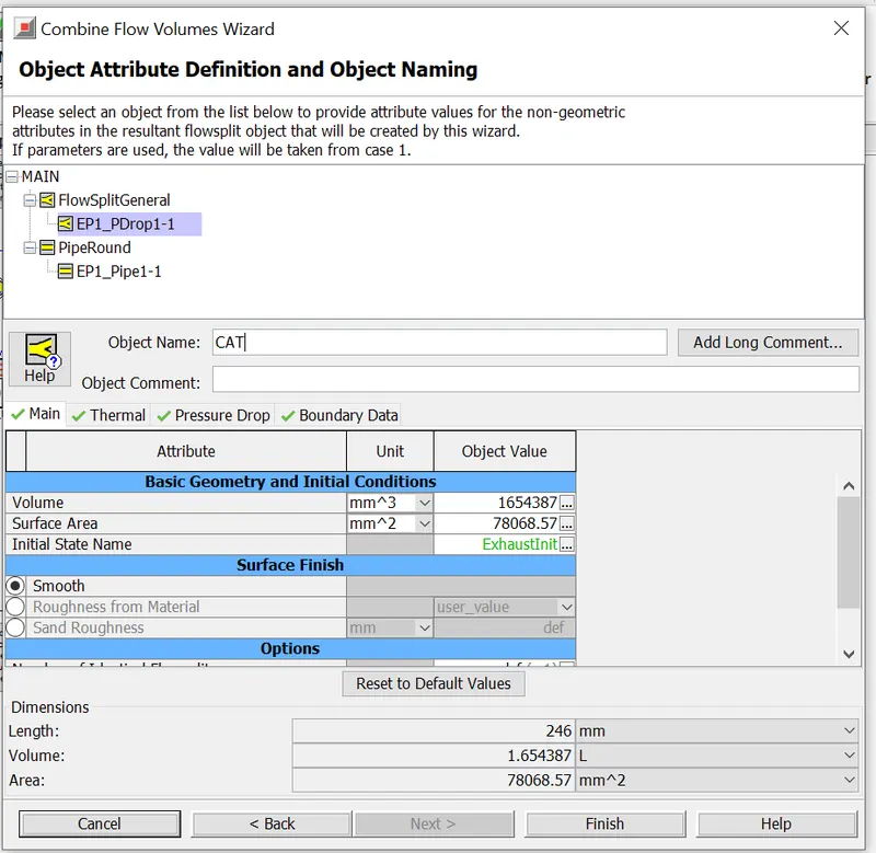
Click "Next" until the last page, "Object Attribute Definition and Object Naming" and select
"EP1_PDrop1-1" to set the object name to "CAT".

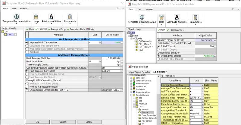
Now, in the combined part CAT-1, replace the wireless signal in the object of Imposed wall temperature with "tav0:CAT-1".

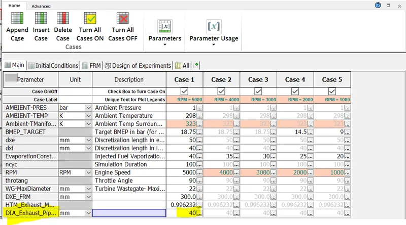
Also assign value of 40 mm to DIA_Exhaust_Pipes_1_Step_2in case setup.

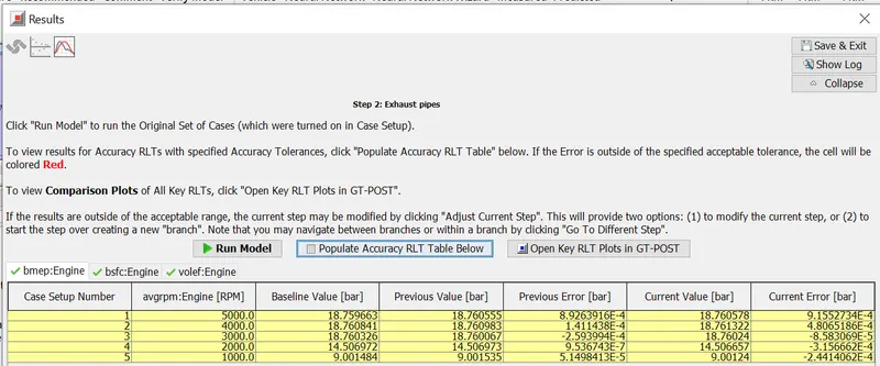
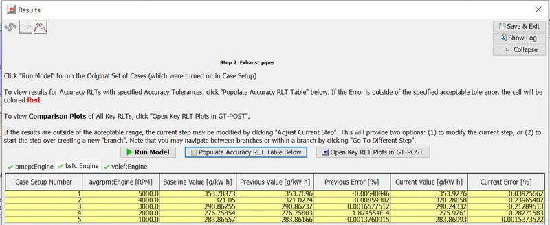
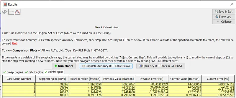
Now click Next (calibration) and "Configure calibration…", set the Response RLT to the trbpoa:Turbine, and set the lower and upper values of the range at 35 and 45 mm, respectively. After running the model for calibration, the results are as follows:

BMEP

BSFC

VOLUMETRIC EFFICIENCY

Step 3:

For step 3 select inlet manifold and follow the same initial steps as earlier.

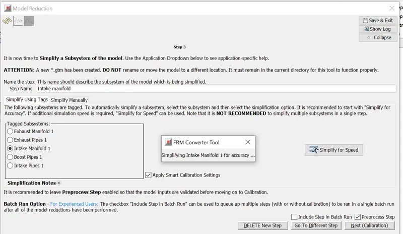
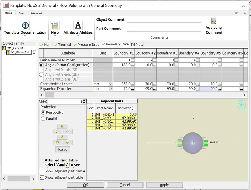
Modify the boundary data in combined inlet manifold.

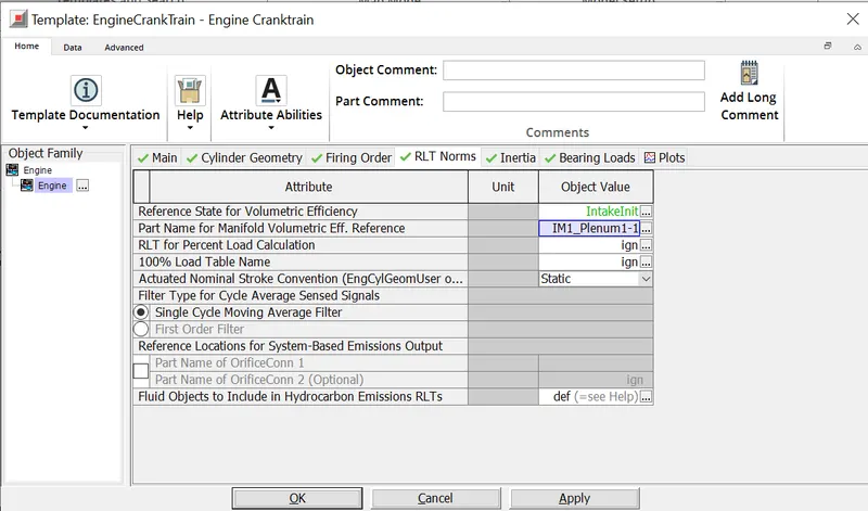
Also, modify the reference values for the part name of inlet manifold.

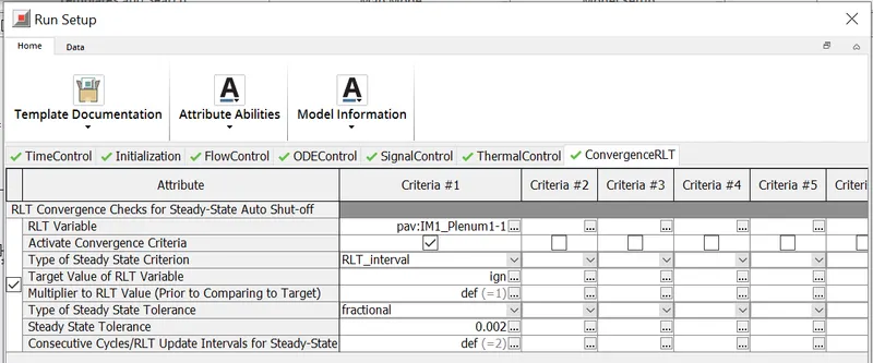
Change the RLT variable in Convergence RLT of Run Setup.

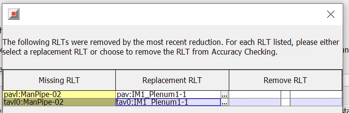
The replacement RLT's are mentioned

Calibration settings of the inlet manifold are as follows:

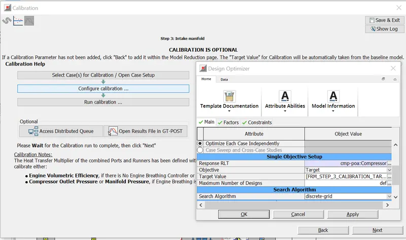
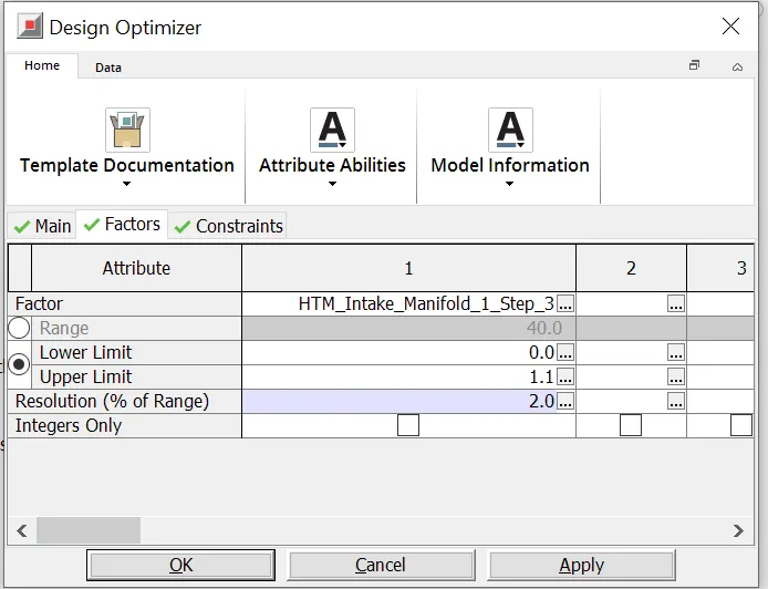
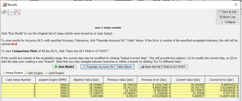
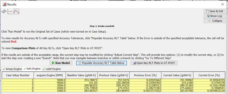
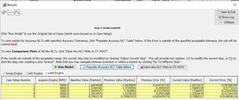
Once the calibration parameters are set, the simulation is performed and the results are as follows:

BMEP

BSFC

VOLUMETRIC EFFICIENCY

Step 4:

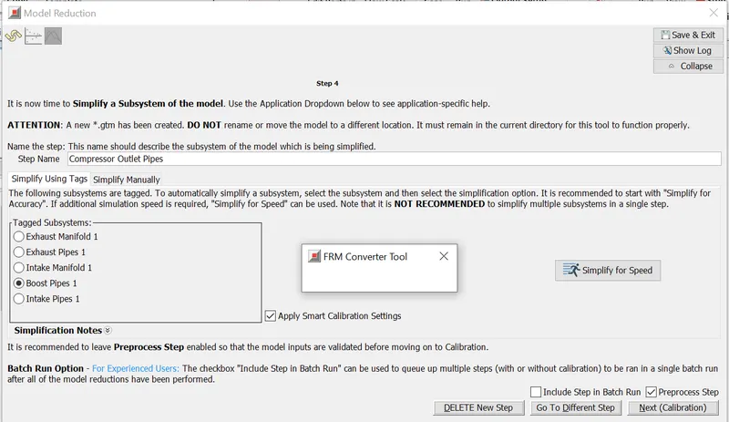
Boost pipes should be selected in this step and named as Compressor Outlet Pipes. Same procedure is followed as previous steps initially.

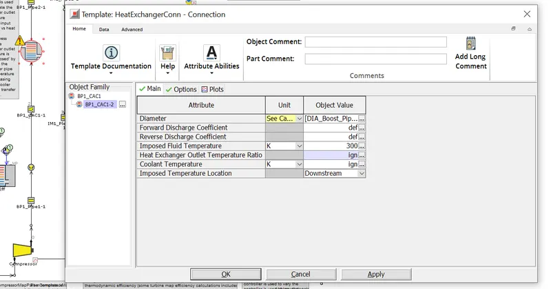
Now, imposed fluid temperature is set as 300 for intercooler and flowsplit.

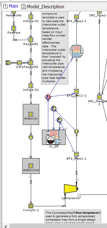
Connect the Control links, sensing Upstream Temperature from "BP1_Pipe1-1" Pipe and Upstream Mass Flow Rate from the "6" OrificeConn upstream of the "BP1_CAC1-1" Flowsplit, and sending the actuator output to both "BP1_CAC1-1" Flowsplit (actuating Wall Temperature) and to the HeatExchangerConn (actuating Imposed Fluid Temperature)

Also, set the value of [DIA_Boost_Pipes_1_Step_4] to 35 mm as an initial value.

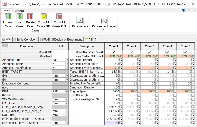
In the Calibration page, select Case 1 for calibration. Under "Configure calibration…", leave the response RLT as the Compressor Massflow-Averaged Outlet Pressure (cmp-poa:Compressor) and set the lower and upper values of the range for DIA_Boost_Pipes_1_Step_4 at 30 and 40 mm. After running the simulation, the results are as follows:

BMEP

BSFC

VOLUMETRIC EFFICIENCY

Step 5:

Name the step "Intake Pipes". Select Intake Pipes 1 from the Tagged Subsystems list. Click on "Simplify for Accuracy". Set the value of [DIA_Intake_Pipes_1_Step_5] to 45 mm in the case setup. In the Data tab of toolbar and click "Delete Unused Objects". Then, in the model tree to the left, right-click on the PipeRound template and choose "Edit Parts in Spreadsheet". View the Discretization Length column to assure that only [DXI_FRM] and [DXE_FRM] are used.

At this point, we have a Fast Running Engine Model running with very high accuracy. If the results are satisfactory for a given application, we can exit out of the FRM converter. However, if additional and better results in terms of speed are desired, further changes can be made to the model

Step 6:

This step is similar to step 1, which calibrates the exhaust manifold. But, it uses " simplify for speed" instead of " simplify for accuracy". The results obained will be much faster than the previous step.ç

Step 7:

The final simplification to the model is Cylinder Slaving of the EngCylinder. The calibration process is simlilar to the previous steps. When the final run is complete, the runtime of the
model is expected to be below 1 xRT for all operating conditions (runtime can be affected by the CPU, stored data, monitors etc.,)

• Build FRM Model for following configuration using FRM builder approach (50 marks)
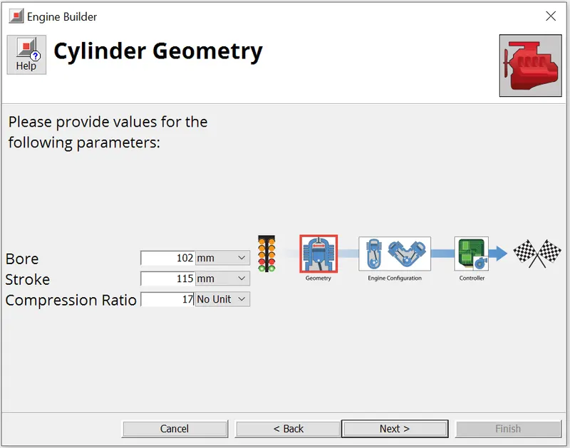
• Bore 102 mm stroke 115 mm CR 17
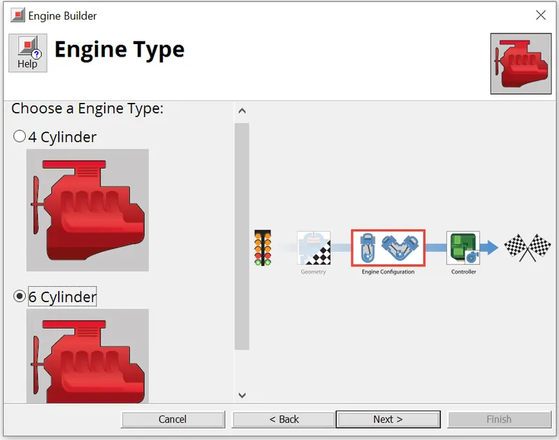
• No of cylinder 6
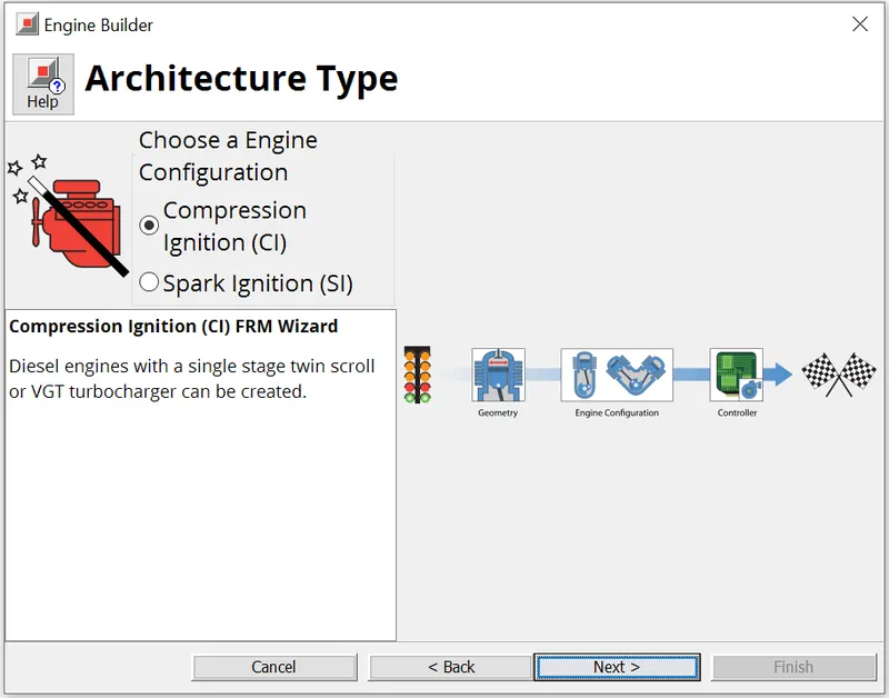
• CI engine
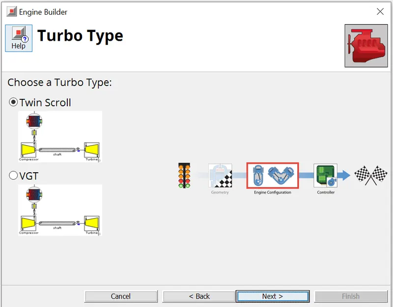
• Twin Scroll Turbine
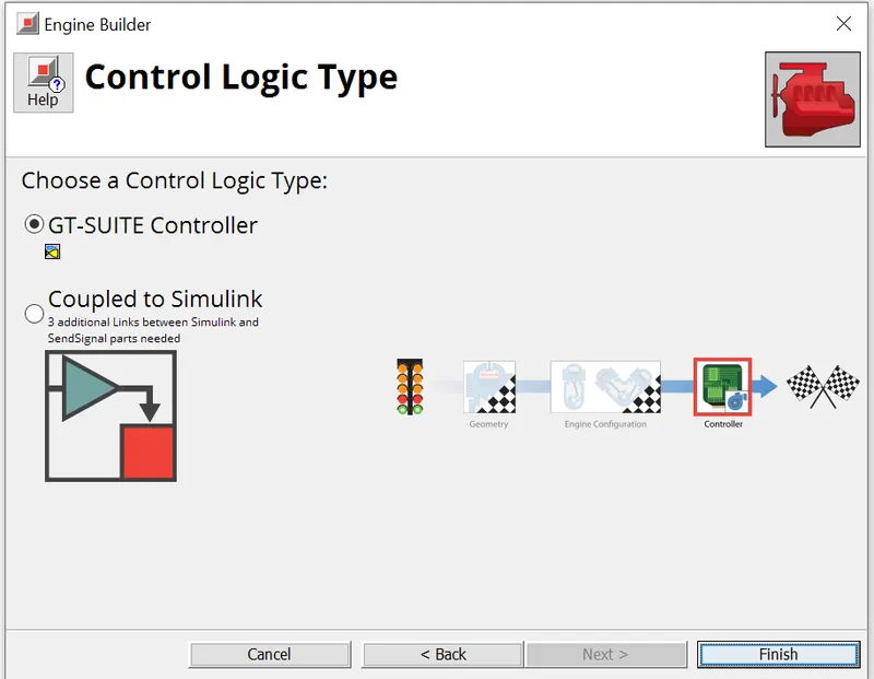
• GT Controller

Initially, select "FRM builder" in the tools section and select "create new engine nodel"

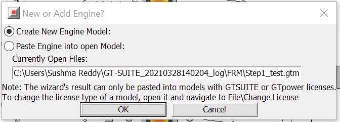
Type of engine

Cylinder geometry with,

• Bore 102 mm stroke 115 mm CR 17

Type of turbo

Number of cylinders

Type of controller

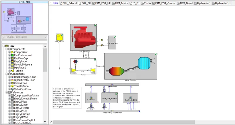
Entire engine model

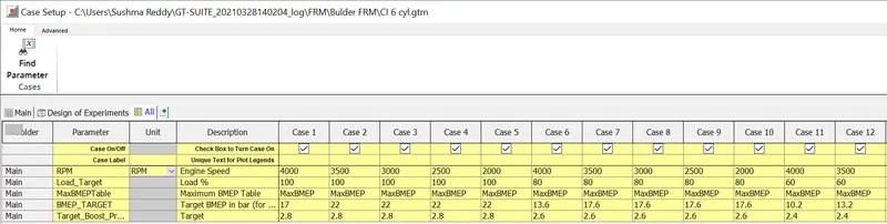
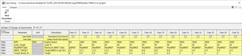
Case setup with all cases selected

Results:

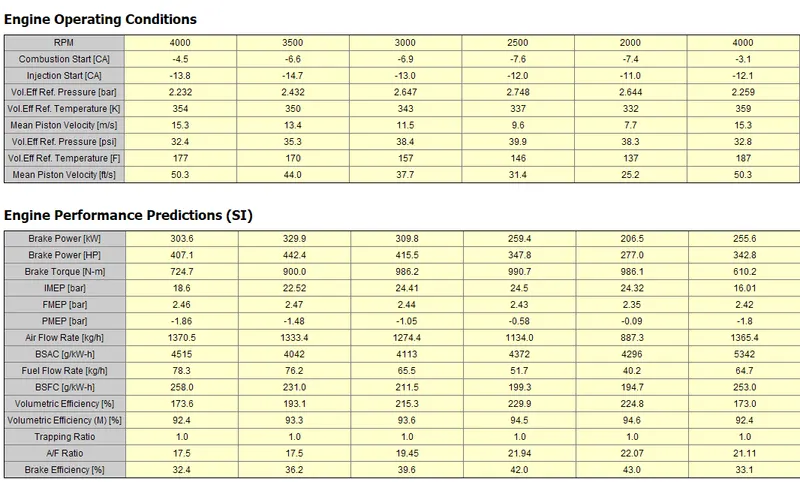
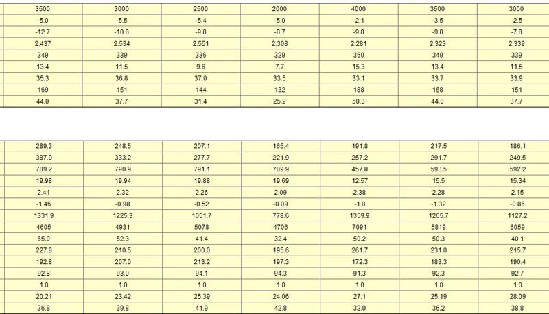
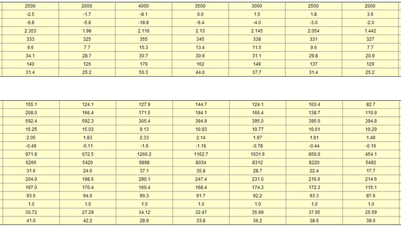
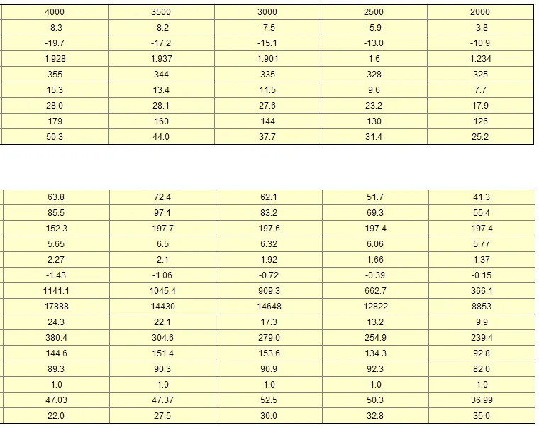
Engine operating conditions and performance:

Simulation duration:

It can be seen that the time interval is varying with various speeds and load conditions. It took very less time for low speed and high load condition.