Week 7 - Auto ignition using Cantera
1.
Objective :
- To understand the variation of Ignition Delay with change of Initial Temparature & Pressure.
- To depict the variation of Mole Fraction of several species with different Initial Temparatures.
Introduction :
We shall consider the Stoichiometric Combustion of Methane, the Chemical Reaction for which, is as follows :
CH4 + 2(O2 + 3.76N2) -> CO2 + 2H2O + 7.52N2
Auto-Ignition Temparature may be defined as the Temperature at which a certain Air-Fuel Mixture spontaneously combusts despite the absence of an external Heat Source & the time at which, this occurs os referred to as Ignition Delay. Auto-Ignition Temperature may depend on a lot of variables, such as Initial Temperature & Pressure, vessel shape & volume, surface activity, contaminants etc. Here, we assume :
Auto-Ignition Temperature [K] = Initial Temperature [K] + 400 [K]
***************************************************************************************************
Case 1 : To study the variation of Auto Ignition characteristics of Methane with varying values of Initial Pressure (1-5 atm), while Initial Temperature is held constant at 1250 K.
Code :
# Program to depict the variation of Auto Ignition characteristics of Methane with
# varying Initial Pressure (1-5 atm), while Initial Temparature is held constant (1250 K)

"""
CH4 + 2(O2 + 3.76N2) -> CO2 + 2H2O + 7.52N2

We shall employ Cantera's Ideal Gas Reactor Model & run the Simulation for 10 seconds

We assume the following :
Auto-Ignition occurs when the Reactor Temparature reaches (T_initial + 400) Kelvin

"""
import numpy as np
import cantera as ct
import matplotlib.pyplot as plt

gas = ct.Solution('gri30.xml')

pressure_range = np.linspace(1, 5, 5)

# The following Array will store the values Ignition Delay for each Temparature
ignition_delay = []

#######################################################################################

# Loop 1 : Looping through Range of Pressures
for i in pressure_range :

    # Specifying the Initial Conditions
    gas.TPX = 1250, i*101325, {'CH4' : 1, 'O2' : 2, 'N2' : 7.52}

    # In the Ideal Gas Reactor Model, T is used instead of the Total Internal Energy U
    # as a State Variable
    reac = ct.IdealGasReactor(gas)

    # The following creates a Network of Reactors for the purpose of Time Integration
    reac_net = ct.ReactorNet([reac])

    # The SolutionArray Class helps organize output data. Additionally, we want time in
    # milli seconds
    states = ct.SolutionArray(gas, extra = ['t_ms', 't'])
    time = 0
    counter = 0

    # Loop 2 : Time Integration Loop
    for j in range(0, 10000) :

        # This is the final time, rather than time-step. For each value of j, our
        # simulaton will advance to the updated value of final time
        time += 1e-3

        # The Advance Method in Cantera calculates the State of our System at the
        #specified final time. Cantera uses an appropriate time-step on it's own
        reac_net.advance(time)

        # Here, we append the results into the states object
        states.append(reac.thermo.state, t_ms = time*1e3, t = time)

        # For each loop, we assign the calculated Temparature to a new variable
        T_new = states.T

        # This if statement is used to determine when Auto-Ignition first occurs
        # We are only interested in the first instance when Ignition occurs &
        # hence the use of the counter
        if (T_new[j] - 1250 > 400 and counter==0) :
            ignition_delay.append(time * 1e3)
            counter += 1
        # End of Loop 2

    # Plotting Temparature VS Time(in ms)
    plt.figure(1)
    plt.plot(states.t_ms, states.T)
    plt.grid('on')
    plt.legend([str(P) + '[atm]' for P in pressure_range])
    plt.xlabel('Time [ms]', fontsize = 13, fontweight = 'bold')
    plt.ylabel('Temparature [K]', fontsize = 13, fontweight = 'bold')
    plt.title('Auto-Ignition Characteristics of Methane with different \n Initial
    Pressures (Initial Temparature = 1250 K)', fontsize = 15, fontweight = 'bold')
# End of Loop 1

#######################################################################################

# Plotting Ignition Delay(in ms) VS Initial Temparature
plt.figure(2)
plt.plot(pressure_range, ignition_delay, '-o')
plt.grid('on')
plt.xlabel('Pressure [atm]', fontsize = 13, fontweight = 'bold')
plt.ylabel('Ignition Delay [ms]', fontsize = 13, fontweight = 'bold')
plt.title('Variation of Ignition Delay with Initial \n Pressure (Initial Temparature = 1250 K)', fontsize = 15, fontweight = 'bold')

plt.show()
Results :
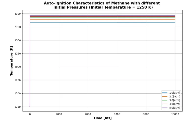
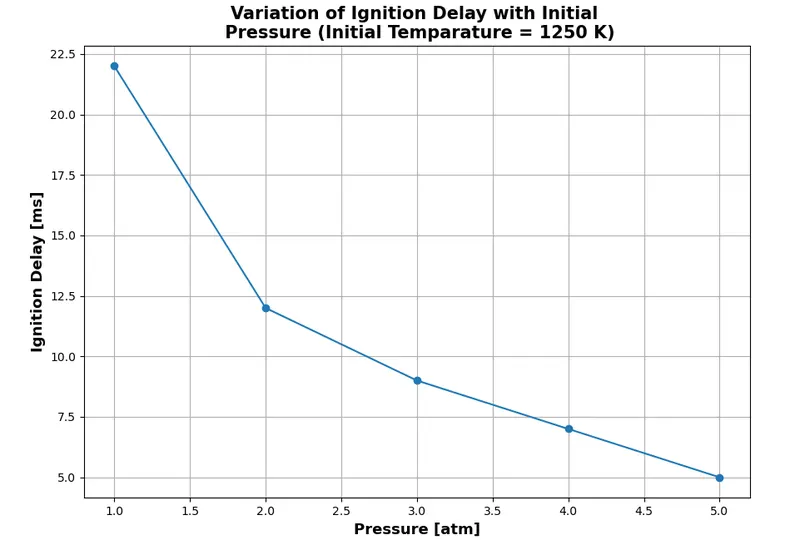
Observations :
It can be observed that Igniton Delay exponentially decreases with increasing Initial Pressure. This can be attributed to the fact that, higher Initial Pressures accelerate the Chemical Kinetics that lead to Auto-Ignition. Furthermore, higher Initial Pressures result in higher Maximum Temparatures. Therefore, Ignition delay heavily depends on Initial Pressure of the System.
***************************************************************************************************
Case 2 : To study the variation of Auto Ignition characteristics of Methane with varying values of Initial Temperature (950-1450 K), while Initial Pressure is held constant at 5 atm.
Code :
# Program to depict the variation of Auto Ignition characteristics of Methane with
# varying Initial Temparature (950 - 1450 K), while Initial Pressure is held constant (5 atm)

"""
CH4 + 2(O2 + 3.76N2) -> CO2 + 2H2O + 7.52N2

We shall employ Cantera's Ideal Gas Reactor Model & run the Simulation for 10 seconds

We assume the following :
Auto-Ignition occurs when the Reactor Temparature reaches (T_initial + 400) Kelvin

"""
import numpy as np
import cantera as ct
import matplotlib.pyplot as plt

gas = ct.Solution('gri30.xml')

temparature_range = np.linspace(950, 1450, 5)

# The following Array will store the values Ignition Delay for each Temparature
ignition_delay = []

#######################################################################################

# Loop 1 : Looping through Range of Temparatures
for i in temparature_range :

    # Specifying the Initial Conditions
    gas.TPX = i, 5*101325, {'CH4' : 1, 'O2' : 2, 'N2' : 7.52}

    # In the Ideal Gas Reactor Model, T is used instead of the Total Internal Energy U
    # as a State Variable
    reac = ct.IdealGasReactor(gas)

    # The following creates a Network of Reactors for the purpose of Time Integration
    reac_net = ct.ReactorNet([reac])

    # The SolutionArray Class helps organize output data. Additionally, we want time in
    # milli seconds
    states = ct.SolutionArray(gas, extra = ['t_ms', 't'])
    time = 0

    # The counter has been used to ensure that, only the first value of Ignition Delay
    # is inserted into the Array
    counter = 0

    # Loop 2 : Time Integration Loop
    for j in range(0, 10000) :

        # This is the final time, rather than time-step. For each value of j, our
        # simulaton will advance to the updated value of final time
        time += 1e-3

        # The Advance Method in Cantera calculates the State of our System at the
        # specified final time. Cantera uses an appropriate time-step on it's own
        reac_net.advance(time)

        # Here, we append the results into the states object
        states.append(reac.thermo.state, t_ms = time*1e3, t = time)

        # For each loop, we assign the calculated Temparature to a new variable
        T_new = states.T

        # This if statement is used to determine when Auto-Ignition first occurs
        # We are only interested in the first instance when Ignition occurs &
        # hence the use of the counter
        if (T_new[j] - 1250 > 400 and counter==0) :
            ignition_delay.append(time * 1e3)
            counter += 1
        # End of Loop 2

    # Plotting Temparature VS Time(in ms)
    plt.figure(1)
    plt.plot(states.t_ms, states.T)
    plt.grid('on')
    plt.legend([str(T) + '[K]' for T in temparature_range])
    plt.xlabel('Time [ms]', fontsize = 13, fontweight = 'bold')
    plt.ylabel('Temparature [K]', fontsize = 13, fontweight = 'bold')
    plt.title('Auto-Ignition Characteristics of Methane with different \n Initial
    Temparatures (Initial Pressure = 5 atm)', fontsize = 15, fontweight = 'bold')
# End of Loop 1

#######################################################################################

# Plotting Ignition Delay(in ms) VS Initial Temparature
plt.figure(2)
plt.plot(temparature_range, ignition_delay, '-o', color = 'black')
plt.grid('on')
plt.xlabel('Temparature [K]', fontsize = 13, fontweight = 'bold')
plt.ylabel('Ignition Delay [ms]', fontsize = 13, fontweight = 'bold')
plt.title('Variation of Ignition Delay with Initial \n Temparature (Initial Pressure = 5 atm)', fontsize = 15, fontweight = 'bold')

plt.show()
Results :
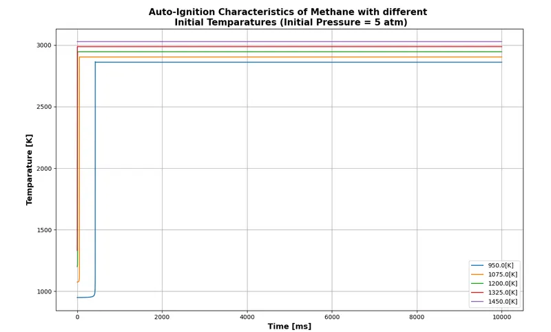
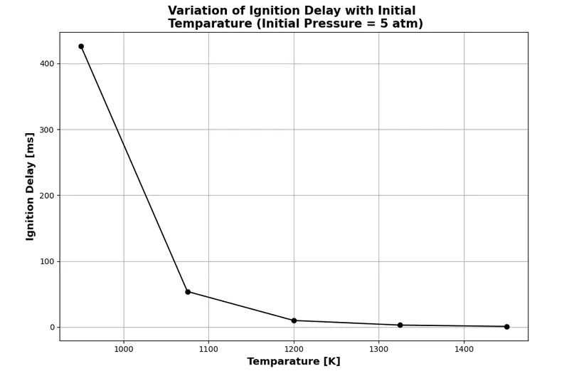
Observations :
We can observe that Ignition Delay drops rapidly with an increase in Initial Temperature, which results in increased Internal Energy & therefore higher Maximum Temperatures. It is interesting to note that there is very little Ignition Delay in case of [Initial Conditions = 1450 K, 5 atm], which implies almost instant auto-ignition.
***************************************************************************************************
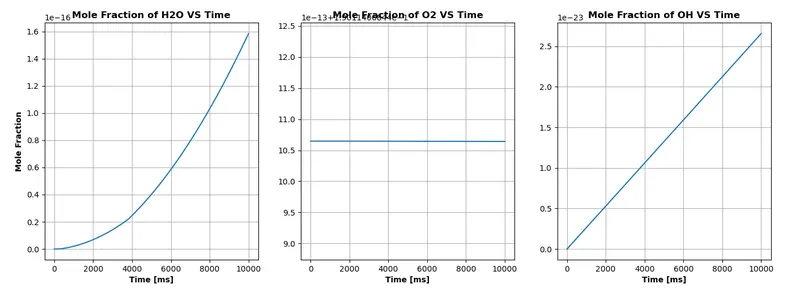
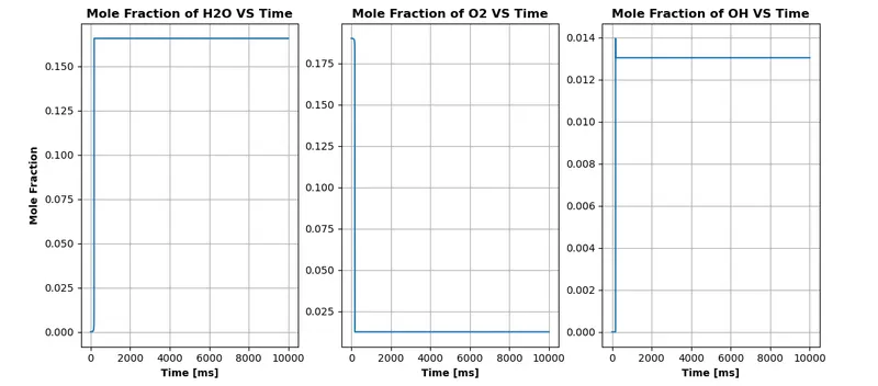
Case 3 : To study the Rate of Change of Molar Concentrations of H2O, O2 & OH for the Initial Temperatures of 500 & 1000 K, while Initial Pressure is held constant at 5 atm.
Code :
# Program to study the Rate of Change of Molar Concentrations of H2O, O2 & OH for the
# Initial Temparatures of 500 & 1000 K, while Initial Pressure is held constant (5 atm)

"""
CH4 + 2(O2 + 3.76N2) -> CO2 + 2H2O + 7.52N2

We shall employ Cantera's Ideal Gas Reactor Model & run the Simulation for 10 seconds

We assume the following :
Auto-Ignition occurs when the Reactor Temparature reaches (T_initial + 400) Kelvin

"""
import numpy as np
import cantera as ct
import matplotlib.pyplot as plt

gas = ct.Solution('gri30.xml')

Temparature_range = [500, 1000]

#######################################################################################

# Loop 1 : Looping through Range of Temparatures
for i in Temparature_range :

    # Specifying the Initial Conditions
    gas.TPX = i, 5*ct.one_atm, {'CH4' : 1, 'O2' : 2, 'N2' : 7.52}

    # In the Ideal Gas Reactor Model, T is used instead of the Total Internal Energy U
    # as a State Variable
    reactor = ct.IdealGasReactor(gas)

    # The following creates a Network of Reactors for the purpose of Time Integration
    reactor_network = ct.ReactorNet([reactor])

    # The SolutionArray Class helps organize output data. Additionally, we want time in
    # milli seconds
    states = ct.SolutionArray(gas, extra = ['t_ms', 't'])
    time = 0

    # Loop 2 : Time Integration Loop
    for j in range(0, 10000) :

        time += 1e-3
        reactor_network.advance(time)
        states.append(reactor.thermo.state, t_ms = time*1e3, t = time)
    # End of Loop 2

    plt.subplot(1, 3, 1)    # plt.subplot(n_rows, n_columns, index)
    plt.plot(states.t_ms, states.X[:, gas.species_index('H2O')])
    plt.grid('on')
    plt.xlabel('Time [ms]', fontsize = 10, fontweight = 'bold')
    plt.ylabel('Mole Fraction', fontsize = 10, fontweight = 'bold')
    plt.title('Mole Fraction of H2O VS Time', fontsize = 12, fontweight = 'bold')

    plt.subplot(1, 3, 2)
    plt.plot(states.t_ms, states.X[:, gas.species_index('O2')])
    plt.grid('on')
    plt.xlabel('Time [ms]', fontsize = 10, fontweight = 'bold')
    plt.title('Mole Fraction of O2 VS Time', fontsize = 12, fontweight = 'bold')

    plt.subplot(1, 3, 3)
    plt.plot(states.t_ms, states.X[:, gas.species_index('OH')])
    plt.grid('on')
    plt.xlabel('Time [ms]', fontsize = 10, fontweight = 'bold')
    plt.title('Mole Fraction of OH VS Time', fontsize = 12, fontweight = 'bold')

    plt.show()
# End of Loop 1
Results :
At 500K & 5 atm:
At 1000 K & 5 atm :
Observations :
In case of 1000K, we observe a sharp increase in the Mole Fractions of H2O & OH, as well as rapid drease in that of O2, which clearly signifies the occurence of Combustion. In the case of 500K, however, we see very little change in the concentrations of either of those species. This must be due to the fact that Auto-Ignition did not take place at all, because of Insuffiecient Temperature. Whatever little change we see, can be attributed to the fact that both H2O & OH have single bonds, which require less energy to break than a double bond, such as in O2. Therefore, analyzing the final species concentrations give us an idea about the phenomenon.
***************************************************************************************************
Conclusion :
We can conclude that Ignition Delay is a strong function of both Initial Temperature & Pressure.