Project 1- Creating your own openFOAM solver

PROJECT 1 : Adding Passive Scalar Transport Equation to icoFoam (icoFoam -> scalarFOAM)

Introduction :

icoFoam is a transient solver for incompressible & laminar flows. It solves the Navier-Stoke's equation using the PISO (Pressure Implicit with Splitting of Operators) algorithm. The need of Pressure-Velocity Coupling Algorithms like SIMPLE & PISO arise from the fact that there is no Transport Equation for Pressure. Our objective here is to add an additional Passive Scalar Transport Equation to this solver, followed by running the Cavity Tutorial with the modified solver.

Modifying icoFoam :

I copy icoFoam to my run directory and rename it as scalarFOAM, followed by appropriate changes to the name of the .C file, along with Make/files (here, we rename the executable to be scalarFOAM & specify the path in which it is to be stored). Furthermore, I make the following changes to the following files :

scalarFOAM.C :

This contains the source code of the solver. This is where we need to code in the Passive Scalar Transport Equation. We do so by adding the following piece of code after the end of the PISO loop :

//Passive scalar transport equation
        fvScalarMatrix sEqn
        (
            fvm::ddt(s)                    //time derivative
           +fvm::div(phi, s)              //convection term
           -fvm::laplacian(su, s)        //diffusion term
        );

        sEqn.relax();                  
        sEqn.solve();

Here, we are solving for a scalar s. The LHS of the sEqn is stored in an fvScalarMatrix, inside which, all the terms (time derivative, convection & diffusion) are treated implicitly (as a part of the fvm namespace, which returns Matrices). Following this, we apply relaxations on it based on user input and finally solve it (equate to 0). In the LHS, the first term is fairly simple, being the time derivative of the scalar s, followed by the linearized convection term (done via Gauss Divergence Theorem, wherein the volume integral of the divergence of the vector field is converted into a surface integral of that vector, which is the flux phi) & finally the diffusion term, along with a diffusion coefficient su. The diffusion term is substracted from the LHS. We have included in the above code two new variables s and su, both of which need to be read from the appropriate dictionaries, which brings us to the next step.

createFields.H :

This is where all the IOobjects reside. For the diffusion coefficient su, I create a dimensionedScalar su, that is to be read from the transportProperties dictionary using the following code :

dimensionedScalar su
(
    "su",
    dimViscosity,
    transportProperties.lookup("su")
);

This code is inserted along side dimensionedScalar nu, which has the same dimensions as su. Now, we create a volumeScalarField s ( which takes in as arguments the IOobject as well as the mesh object), using the following code :

Info<< "Reading field s\n" << endl;
volScalarField s
(
    IOobject
    (
        "s",
        runTime.timeName(),
        mesh,
        IOobject::MUST_READ,
        IOobject::AUTO_WRITE
    ),
    mesh
);

This concludes the step of modifying the solver. All that remains is running wmake to create scalarFOAM.so. Now, we shall try to validate the custom solver by running the Cavity test case.

Running Cavity using scalarFOAM :

I copy the Cavity tutorial in my run directory & rename it scalarCavity.

Pre-Processing :

0/s :

I copy the p file and rename it s. Inside, I specify that my scalar field is dimensionless and that it has a default internal field value of 0. I use the following code :

dimensions      [0 0 0 0 0 0 0];

internalField   uniform 0;

boundaryField
{
    movingWall
    {
        type            zeroGradient;
    }

    fixedWalls
    {
        type            zeroGradient;
    }

    frontAndBack
    {
        type            empty;
    }
}

constant/transportProperties :

This is the dictionary from which su is to be read, for which I specify it's dimensionSet and value. Therefore, I add the following :

su              [0 2 -1 0 0 0 0] 0.0001;

system/controlDict :

Here, we must specify our custom solver (scalarFOAM) in the application field. Along with this, I change the endTime to 7 seconds.

system/blockMeshDict :

Here, we specify the number of cells in each direction, (50*50) in this case.

blocks
(
    hex (0 1 2 3 4 5 6 7) (50 50 1) simpleGrading (1 1 1)
);

system/fvSchemes :

This where we must specify the schemes to be used for solving the following terms : fvm::div(phi, s) & fvm::laplacian(su, s). I use Gauss Upwind for the divergence term & Gauss Linear Corrected for the Laplacian term.

divSchemes
{
    default         none;
    div(phi,U)      Gauss linear;
    div(phi,s)      Gauss upwind;
}

laplacianSchemes
{
    default         Gauss linear corrected;
}

system/fvSolution :

Here, we must specify the particular Linear Solver that is to be used for solving our scalar matrix. We cannot use the exact same solver for our scalar, which is specified as default for the pressure, i.e, PCG. This is because, PCG is meant for symmetric matrices, PBiCG for asymmetric matrices & smoothSolver for any of those.

p
{
    solver          PCG;
    preconditioner  DIC;
    tolerance       1e-06;
    relTol          0.05;
}

s
{
    solver          smoothSolver;
    smoother        symGaussSeidel;
    tolerance       1e-05;
    relTol          0;
}

system/setFieldsDict :

I this file file from the Dam Break tutorial & make the appropriate changes. Here, I want to define a field (a sphere at the centre of the domain) for s in the domain. Inside the field, the scalar will have a value 1. Everywhere else, it will be 0. This is done with the help of the following code :

defaultFieldValues
(
    volScalarFieldValue s 0
);

regions
(
    sphereToCell
    {
    	centre (0.05 0.05 0);
    	radius 0.03;
        
        fieldValues
        (
            volScalarFieldValue s 1
        );
    }
);

Running the Simulation :

The objective of this simulation is to observe the change in our scalar field s (say a blob of ink), with time, in the Cavity setup (fixed bottom wall & moving top wall). Now all that remains are executing the following commands in the Terminal :

blockMesh : This will create the mesh as specified in blockMeshDict.

setFields : This will set the fields as specified in setFieldsDict.

scalarFOAM : This will run the simulation.

This being a small simulation, is completed in under a minute.

Post-Processing :

After the simulation is complete, I create an empty file named foam.foam and type the following code in the terminal : paraview foam.foam &. This opens up the solution in ParaView. The animation shows expected results, i.e, the ink blob rotates and is smeared away due to the moving top wall. The following will help visualize it better :

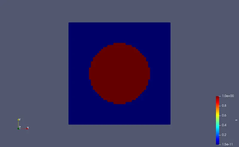at t = 0 s

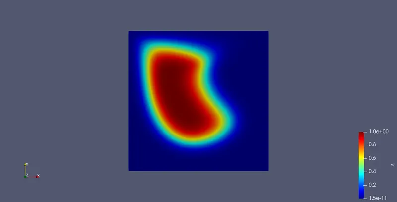at t = 0.1 s

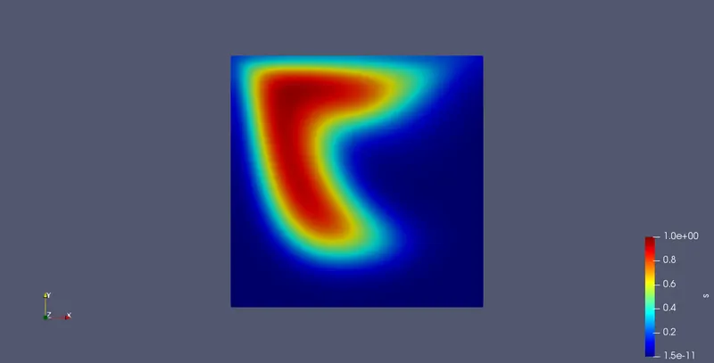at t = 0.2 s

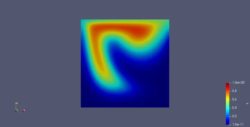at t = 0.3 s

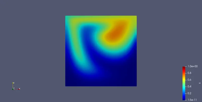at t = 0.4 s

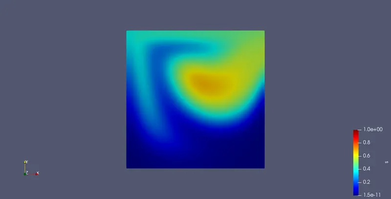at t = 0.5 s

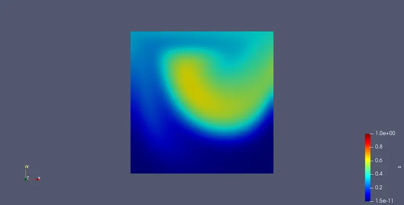at t= 0.6 s

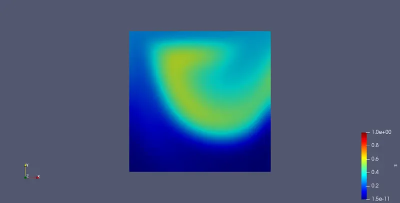at t = 0.7 s

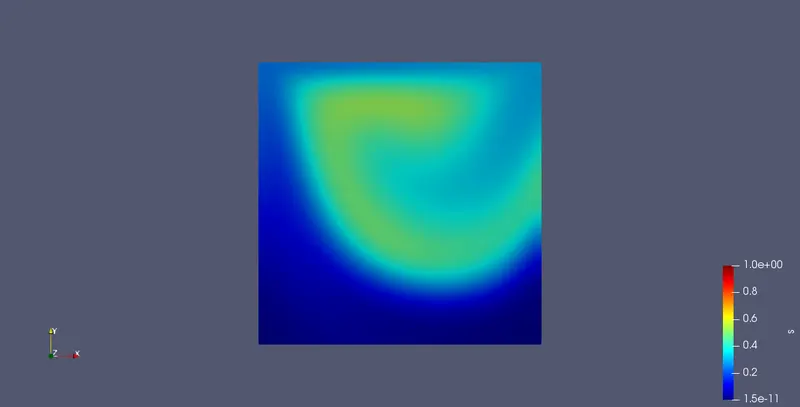at t = 0.8 s

Conclusion :

This simple simulation sheds light into the basic steps involving addition of Passive Scalar Transport Equation to IcoFoam & testing it using the Cavity Tutorial.

Platform : openFoam-v8 -> Ubuntu 20.04 -> VirtualBox -> Windows 10

Source : https://www.youtube.com/watch?v=L94iYGvZr9Q&list=LL&index=6