Week 7 - Auto ignition using Cantera

AIM

The aim of this challenge is to simulate the autoignition temperature for methane.

Problem Statement:

PART I

Use the same reactor network code as shown in the video to simulate the Auto Ignition Time for Methane under the following conditions, (simulation time = 10 secs)

1. Plot the variation of Auto Ignition time of Methane with a constant temperature of 1250K and

pressure varying from 1 to 5 atm.

2. Plot the variation of Auto Ignition time of Methane with a constant pressure of 5 atm and temperature varying from 950K to 1450K.

PART II

Further, observe and print the rate of change of molar concentrations of the given elements "H2O, O2, OH" with respect to the time, (simulation time = 10 secs)

Explain the behavior of the graph for 2 cases,

When Temperature is 1000K and pressure 5 bar

When Temperature is 500K and pressure 5 bar

NOTE:

Auto Ignition time is the time when the temperature of the reactor is Initial Temperature plus 400K.

Python Program:

""" PART I

Use the same reactor network code as shown in the video to simulate the Auto Ignition Time for Methane under the following conditions, (simulation time = 10 secs)
1. Plot the variation of Auto Ignition time of Methane with a constant temperature of 1250K and 
pressure varying from 1 to 5 atm.
2. Plot the variation of Auto Ignition time of Methane with a constant pressure of 5 atm 
and temperature varying from 950K to 1450K.

NOTE:

Auto Ignition time is the time when the temperature of the reactor is Initial Temperature plus 400K.

"""
import matplotlib.pyplot as plt
import cantera as ct
import numpy as np

def cv_combust(T,P,species_dist):

	gas = ct.Solution('gri30.xml')
	gas.TPX = T,P,species_dist
	r = ct.IdealGasReactor(gas)
	sim = ct.ReactorNet([r])
	time = 0.0
	state = ct.SolutionArray(gas,extra = ['time_in_ms' , 't'])

	for n in range(10000):
		time += 1e-3
		sim.advance(time)
		state.append(r.thermo.state,time_in_ms = time * 1e3, t = time)

	return state

X = {'CH4' :1 ,'O2' : 2 , 'N2' : 7.52}			# input chemical composition
temp_varication = np.linspace(950,1450,11) #temperature varaction between 950 K to 1450 K
pressure_varaction = np.linspace(1,5,6)		# pressure varaction between 1bar to 5bar
ignition_delay_temp = []
ignition_delay_pressure = []

# cv_combust(1400,101325,{'CH4' :1 ,'O2' : 2 , 'N2' : 7.52})
for i in range(11):							# loop for temperature varaction
	new_temp_state = cv_combust(temp_varication[i],5*101325, X)
	print(new_temp_state.T)
	print(len(new_temp_state.T))
	plt.figure(6)
	plt.plot(new_temp_state.T)
	plt.xlabel('Number of timesteps')
	plt.ylabel('Temperature')
	plt.title('Variation of Auto-ignition Temperature with inlet Temperature')
	plt.legend(temp_varication)
	for n in range(10000):
		if (new_temp_state.T[n] - temp_varication[i]) >= 400:
		# ignition_delay = new_temp_state.time_in_ms
			ignition_delay_temp.append(new_temp_state.time_in_ms[n])
			break

print(ignition_delay_temp)

for i in range(6):							# loop for temperature varaction
	new_pressure_state = cv_combust(1250,pressure_varaction[i]*101325, X)
	print(new_pressure_state.T)
	print(len(new_pressure_state.T))
	plt.figure(3)
	plt.plot(new_pressure_state.T)
	plt.xlabel('Number of timesteps')
	plt.ylabel('Temperature')
	plt.title('Variation of Auto-ignition Temperature with inlet Pressure')
	plt.legend(['1 Bar','2 Bar', '3 Bar','4 Bar', '5 Bar'])
	for n in range(10000):
		if (new_pressure_state.T[n] - 1250) >= 400:
		# ignition_delay = new_temp_state.time_in_ms
			ignition_delay_pressure.append(new_pressure_state.time_in_ms[n])
			break

print(ignition_delay_pressure)



"""
PART II

Further, observe and print the rate of change of molar concentrations of 
the given elements "H2O, O2, OH" with respect to the time, (simulation time = 10 secs)

Explain the behavior of the graph for 2 cases,

When Temperature is 1000K and pressure 5 bar
When Temperature is 500K and pressure 5 bar
NOTE:

The command to extract mole fractions of a given 'species' is,

states.X[:,gas.species_index('species')])

"""
new_t500 = cv_combust(500,5*101325, X)
print(new_t500.T)
print(len(new_t500.T))
plt.figure(4)
plt.subplot(3, 1, 1)
plt.plot(new_t500.t,new_t500.X[:,new_t500.species_index('H2O')])
plt.xlabel('Time (ms)')
plt.ylabel('H20 Mole Fraction')
plt.subplot(3, 1, 2)
plt.plot(new_t500.t,new_t500.X[:,new_t500.species_index('O2')])
plt.xlabel('Time (ms)')
plt.ylabel('02 Mole Fraction')
plt.subplot(3, 1, 3)
plt.plot(new_t500.t,new_t500.X[:,new_t500.species_index('OH')])
plt.xlabel('Time (ms)')
plt.ylabel('OH Mole Fraction')
plt.tight_layout()

new_t1000 = cv_combust(1000,5*101325, X)
print(new_t1000.T)
print(len(new_t1000.T))
plt.figure(5)
plt.subplot(3, 1, 1)
plt.plot(new_t1000.t,new_t1000.X[:,new_t1000.species_index('H2O')])
plt.xlabel('Time (ms)')
plt.ylabel('H20 Mole Fraction')
plt.subplot(3, 1, 2)
plt.plot(new_t1000.t,new_t1000.X[:,new_t1000.species_index('O2')])
plt.xlabel('Time (ms)')
plt.ylabel('02 Mole Fraction')
plt.subplot(3, 1, 3)
plt.plot(new_t1000.t,new_t1000.X[:,new_t1000.species_index('OH')])
plt.xlabel('Time (ms)')
plt.ylabel('OH Mole Fraction')
plt.tight_layout()

plt.figure(1)
plt.plot(temp_varication,ignition_delay_temp)
plt.xlabel('temp_varication in K')
plt.ylabel('Auto-ignition Time [ms]')
plt.title('Ignition time delay Vs Temperature at pressure 5 bar')

plt.figure(2)
plt.plot(pressure_varaction,ignition_delay_pressure)
plt.xlabel('pressure_varaction in bar')
plt.ylabel('Auto-ignition Time [ms]')
plt.title('Ignition time delay Vs Pressure at 1250 K')

plt.show()

Result:

1. Figure 1 a & b : Plot the variation of Auto Ignition time of Methane with a constant temperature of 1250K and pressure varying from 1 to 5 atm.

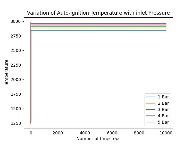
Figure: 1a

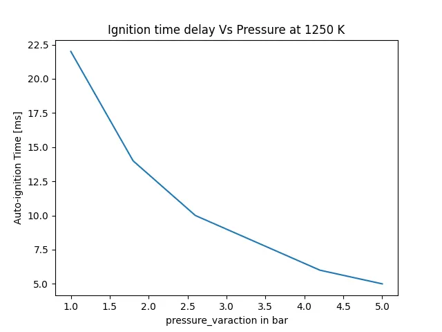
Figure 1b

2. Plot the variation of Auto Ignition time of Methane with a constant pressure of 5 atm and temperature varying from 950K to 1450K.

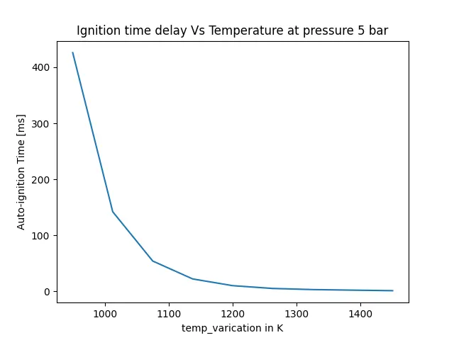
Figure 2 a

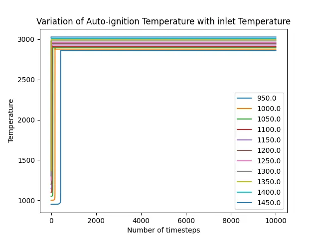
Figure 2b

3. The rate of change of molar concentrations of the given elements "H2O, O2, OH" with respect to the time, (simulation time = 10 secs)

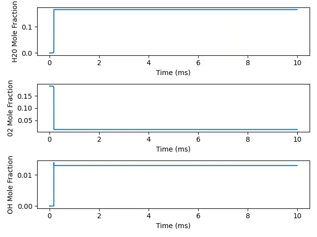
Figure 3: rate of change of molar concentrations of the given elements "H2O, O2, OH" with respect to the time at 1000K, Pressure 5 bar.

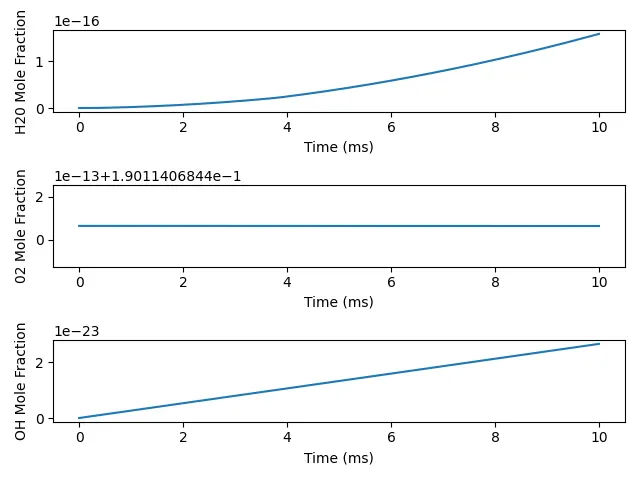
Figure 4: rate of change of molar concentrations of the given elements "H2O, O2, OH" with respect to the time at 500K, Pressure 5 bar.