Week 7 - Auto ignition using Cantera

Auto Ignition:-

The ignition is the process of starting the combustion of fuel in the cylinders of an internal combustion engine. Auto-ignition is the self-ignition of the fuel/air mixture before the spark has fired. This can be caused by hot combustion residuals or hot parts of the cylinder wall. Auto-ignition leads to high temperatures and pressures and also can be harmful to the engine.

Ignition delay(ID) is defined as the time gap between fuel injection into the combustion chamber and the very beginning of its ignition.

Part-I:

1. Plot the variation of Auto Ignition time of Methane with a constant temperature of 1250K and pressure varying from 1 to 5 atm.

Code:

# constant temperature

import sys
import math
import matplotlib.pyplot as plt
import cantera as ct
import numpy as np

gas = ct.Solution('gri30.xml')
press = np.linspace(101325,506625,9)
T=1250
'''
time_s = 0
time_e = 10
time_st = 1e-3
'''
n = 10000
ignition_delay = []


for P in press:
	gas.TPX = T, P, {'CH4':1,'O2':2,'N2':7.52}
	r = ct.IdealGasReactor(gas)
	sim = ct.ReactorNet([r])
	T_old = T
	time = 0

	states = ct.SolutionArray(gas, extra=['time_in_ms','t'])
	print('{:10s} {:10s} {:10s}'.format('t[s]','T[K]','p [atm]'))
	j=1

	for j in range(n):
		time += 1e-3
		sim.advance(time)
		states.append(r.thermo.state,time_in_ms=time*1e3,t=time)
		T_new=states.T
		T_new=T_new[j-1]

		if (T_new>=400+T_old):
			ignition_delay.append(time)
			
			T_old = states.T
			T_old = T_old[j-1]

			print('ignition_delay')



	plt.figure(1)
	plt.plot(states.t,states.T)


	plt.legend(['press = ' + str(T) + '[k]' for P in press])
	plt.xlabel('Time')
	plt.ylabel('pressure')


#print('Ignition_delay = ',ignition_delay)
plt.figure(2)
plt.plot(press/101325,ignition_delay,'-*')
plt.xlabel('pressere in [atm]')
plt.ylabel('Ignition_delay in [ms]')
plt.show()
plt.show()

Plot:

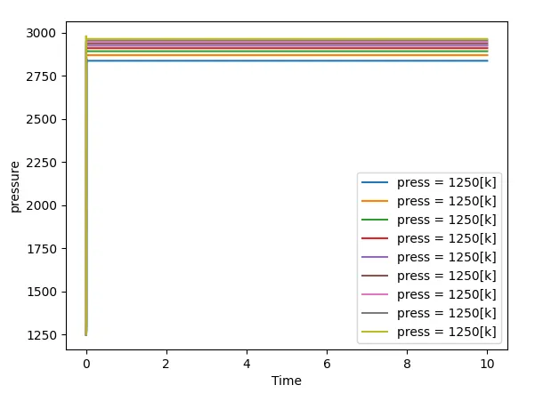
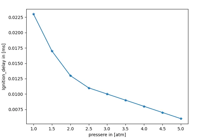
2. Plot the variation of Auto Ignition time of Methane with a constant pressure of 5 atm and temperature varying from 950K to 1450K.

Code:

# constant pressure

import sys
import math
import matplotlib.pyplot as plt
import cantera as ct
import numpy as np

gas = ct.Solution('gri30.xml')
temp = np.linspace(950,1450,6)
n = 10000
ignition_delay = []
states1 = []

for T in temp:
	gas.TPX = T, 5*ct.one_atm, {'CH4':1,'O2':2,'N2':7.52}
	r = ct.IdealGasReactor(gas)
	sim = ct.ReactorNet([r])
	T_old = T
	time = 0

	states = ct.SolutionArray(gas, extra=['time_in_ms','t'])
	print('{:10s} {:10s} {:10s}'.format('t[s]','T[K]','p [atm]'))
	j=1

	for j in range(n):
		time += 1e-3
		sim.advance(time)
		states.append(r.thermo.state,time_in_ms=time*1e3,t=time)
		T_new=states.T
		T_new=T_new[j-1]

		if (T_new>=400+T_old):
			ignition_delay.append(time)
			
			T_old = states.T
			T_old = T_old[j-1]

			print('ignition_delay')



	plt.figure(1)
	plt.plot(states.t,states.T)


plt.legend(['Temp = ' + str(T) + '[k]' for T in temp])
plt.xlabel('Time')
plt.ylabel('Temperature')
print('Ignition_delay = ',ignition_delay)
plt.figure(2)
plt.plot(temp,ignition_delay,'-*')
plt.xlabel('Temperature in [K]')
plt.ylabel('Ignition_delay in [ms]')
plt.show()
plt.show()

Plot:

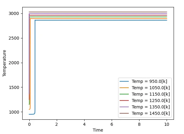
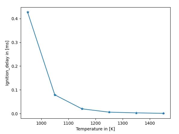
If we increased temperature or pressure at the initial mixture it leads to quicker combustion. The ignition delay decreases with the pressure. Autoignition is more sensitive to temperature, the bigger the initial temperature the lower autoignition time.

Part-II:

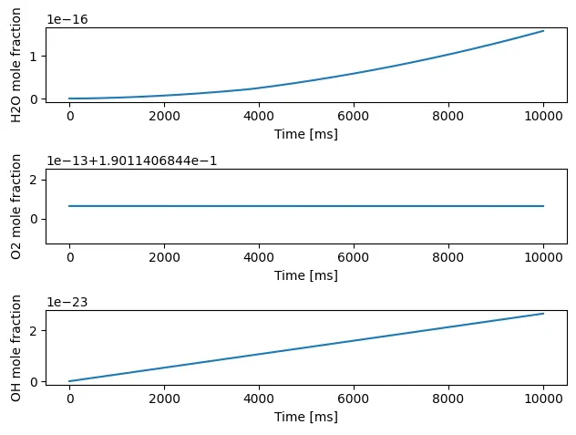
Further, observe and print the rate of change of molar concentrations of the given elements "H2O, O2, OH" with respect to the time, (simulation time = 10 secs):

import sys
import math
import matplotlib.pyplot as plt
import cantera as ct
import numpy as np

gas = ct.Solution('gri30.xml')
temp = [500,1000]
p = ct.one_atm*5

species = {'CH4':1, 'O2':2, 'N2':7.52}

for T in temp:
	gas.TPX = T,p, {'CH4':1, 'O2':2, 'N2':7.52}
	r = ct.IdealGasReactor(gas)
	sim = ct.ReactorNet([r])

	time = 0
	states = ct.SolutionArray(gas,extra=['time_in_ms','t'])
	T_old = T
	time_s = 10*1000
	i = 1
	for i in range(time_s+1):
		time += 1e-3
		sim.advance(time)
		states.append(r.thermo.state,time_in_ms = time*1e3, t=time)

plt.subplot(3,1,1)
plt.plot(states.time_in_ms,states.X[:,gas.species_index('H2O')])
plt.xlabel('Time [ms]')
plt.ylabel('H2O mole fraction')

plt.subplot(3,1,2)
plt.plot(states.time_in_ms,states.X[:,gas.species_index('O2')])
plt.xlabel('Time [ms]')
plt.ylabel('O2 mole fraction')

plt.subplot(3,1,3)
plt.plot(states.time_in_ms,states.X[:,gas.species_index('OH')])
plt.xlabel('Time [ms]')
plt.ylabel('OH mole fraction')
plt.tight_layout()
plt.show()

Plot:

For temp=500k and pre=5bar

For temp=1000k and pre=5bar

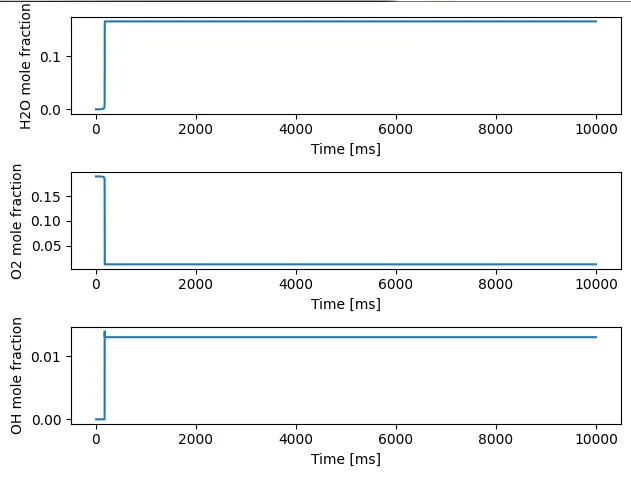
The H2O and OH mole fraction increases and become stable as the autoignition time increases, because H2O and OH are products of methane combustion. O2 decreases because it is a reactant in methane combustion.