Week 6 - Multivariate Newton Rhapson Solver
JORGE LOZANO
Computational Combustion using Python and Cantera
Multivariate Newton Rhapson Solver
Objective
In this challenge, you will solve the set of equations given below,
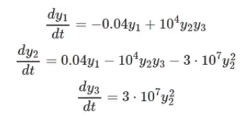
- Incorporate numerical jacobian. That is, the jacobian should be estimated numerically and not analytically.
- Solve the problem using Implicit Euler Method/Backward Differencing, assume the initial conditions as 1 for y1 and 0 for y2 and y3 respectively.
- Take alpha as 1. Run the simulation for 10 minutes.
- Choose a suitable step size and explain the reason for choosing that step size, what is the ideal step size in this case?
Documentation
Newton’s method requires first derivatives. We recall the definition (see calculus in several variables). [1]
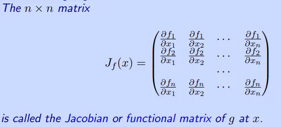
Jacobian: Numerical Computation
Often the Jacobian is not analytically available, and it must be computed numerically. It can be computed column wise by finite differences
In calculus, Newton's method is an iterative method for finding the roots of a differentiable function F, which are solutions to the equation F (x) = 0. In optimization, Newton's method is applied to the derivative f ′ of a twice-differentiable function f to find the roots of the derivative (solutions to f ′(x) = 0), also known as the stationary points. These solutions may be minimal, maxima, or saddle points.
Newton's method, also called the Newton-Raphson method, is a root-finding algorithm that uses the first few terms of the Taylor series of a function f(x) in the vicinity of a suspected root. Newton's method is sometimes also known as Newton's iteration, although in this work the latter term is reserved to the application of Newton's method for computing square roots.[2]
Analysis
A numerical solution will be given, using the Newton-Rhapson solver by which it will be running for 10 minutes, varying the timestep, and having the alpha and initial y values as documented.
The code will be given next:
"""
f1	[dy1/DT]  -0.04*Y1+(10e4)*Y2*Y3=0
f2	[dy2/DT]   0.04*Y1-(10e4)*Y2*Y3-3*(10e7)*Y2^2=0
f3	[dy3/DT]   3*(10e7)*Y2^2=0"""
import numpy as np
import matplotlib.pyplot as plt
from numpy.linalg import inv
#SYSTEM TO SOLVE:
def f1(y1,y2,y3,y_old_1,DT):
	return (y_old_1 + DT*(-0.04*y1 +pow(10,4)*y2*y3) - y1)
def f2(y1,y2,y3,y_old_2,DT):
	return (y_old_2 + DT*(0.04*y1 - (pow(10,4)*y2*y3) - (3*pow(10,7)*y2*y2)) - y2)
def f3(y1,y2,y3,y_old_3,DT):
	return (y_old_3 + DT*(3*pow(10,7)*y2*y2) - y3)
def Jacobian(y1,y2,y3,y_old_1,y_old_2,y_old_3,DT):
	j= np.ones((3,3))
	h = 1e-7#STEP
	j[0,0]= (f1(y1+h,y2,y3,y_old_1,DT)-f1(y1,y2,y3,y_old_1,DT))/h
	j[1,0]= (f2(y1+h,y2,y3,y_old_2,DT)-f2(y1,y2,y3,y_old_2,DT))/h
	j[2,0]= (f3(y1+h,y2,y3,y_old_3,DT)-f3(y1,y2,y3,y_old_3,DT))/h
	j[0,1]= (f1(y1,y2+h,y3,y_old_1,DT)-f1(y1,y2,y3,y_old_1,DT))/h
	j[1,1]= (f2(y1,y2+h,y3,y_old_2,DT)-f2(y1,y2,y3,y_old_2,DT))/h
	j[2,1]= (f3(y1,y2+h,y3,y_old_3,DT)-f3(y1,y2,y3,y_old_3,DT))/h
	j[0,2]= (f1(y1,y2,y3+h,y_old_1,DT)-f1(y1,y2,y3,y_old_1,DT))/h
	j[1,2]= (f2(y1,y2,y3+h,y_old_2,DT)-f2(y1,y2,y3,y_old_2,DT))/h
	j[2,2]= (f3(y1,y2,y3+h,y_old_3,DT)-f3(y1,y2,y3,y_old_3,DT))/h
	return j
y_old_1= 1
y_old_2= 0
y_old_3= 0
y_old= np.ones((3,1))
y_old[0]= y_old_1
y_old[1]= y_old_2
y_old[2]= y_old_3
F= np.copy(y_old)
alpha= 1
t= 600#SECONDS =10 MINS
DT= 1
n= int(t/DT)
y_new1= []
y_new2= []
y_new3= []
it= []
error_new= []
iter= 1
tol= 1e-7

for i in range(0,n):
	error= 1e10
	while error > tol:
		jac= Jacobian(y_old[0],y_old[1],y_old[2],y_old_1,y_old_2,y_old_3,DT)
		F[0]= f1(y_old[0],y_old[1],y_old[2],y_old_1,DT);
		F[1]= f2(y_old[0],y_old[1],y_old[2],y_old_2,DT);
		F[2]= f3(y_old[0],y_old[1],y_old[2],y_old_3,DT);
		y_new = y_old - alpha * np.matmul(inv(jac), F);
		error = np.max(np.abs(y_new-y_old));
		y_old = y_new
	Result= 'iter= {0} error= {1} y1= {2} y2= {3} y3= {4} '.format(iter,error, y_new[0], y_new[1], y_new[2])
	y_old = y_new;
	y_new1.append(y_new[0])
	y_new2.append(y_new[1])
	y_new3.append(y_new[2])
	error_new.append(error)
	iter= iter + 1
	it.append(iter)
	y_old_1= y_new[0]
	y_old_2= y_new[1]
	y_old_3= y_new[2]
print(Result)
plt.style.use('grayscale')
figure,(p1,p2)=plt.subplots(2,1)
plt.yscale("log")
p2.set_xlabel("Iterations (No. Steps)",fontsize = 20)
p1.set_ylabel("Error value",fontsize = 15)
p2.set_ylabel("Error value",fontsize = 15)
p1.set_title("Multivariate Newton Rhapson Solver Dt= "+str(DT),fontsize = 25)
p1.plot(it,y_new1,linewidth=2.5,color='blue',label='Y1 value')
p2.plot(it,y_new2,linewidth=2.5,color='orange',label='Y2 value')
p1.plot(it,y_new3,linewidth=2.5,color='green',label='Y3 value')
p2.plot(it,error_new,linewidth=2.5,color='red',label='Error')
p1.legend()
p2.legend()
p1.grid('TRUE')
p2.grid('TRUE')
plt.show()
Graphs results
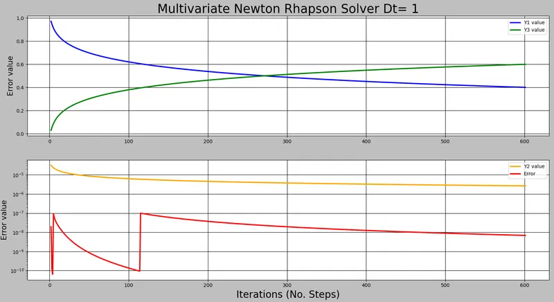
For a timestep of 1:
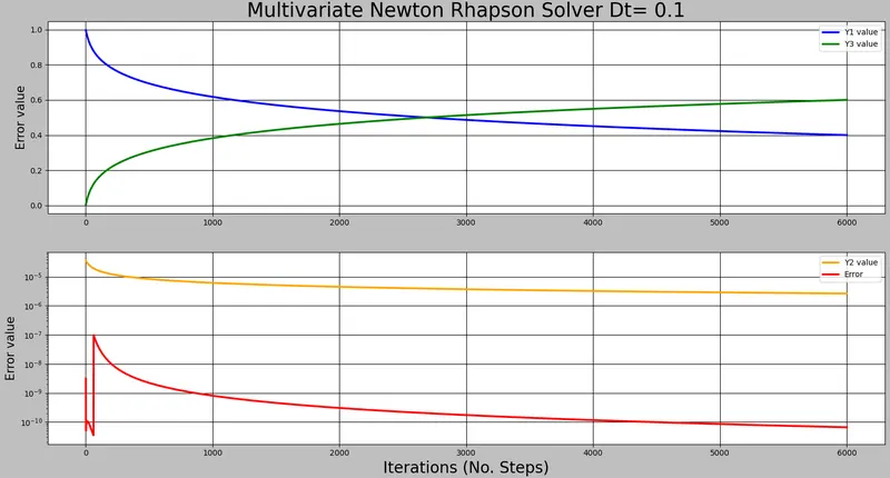
For a timestep of 0.1:
For a timestep of 0.01:
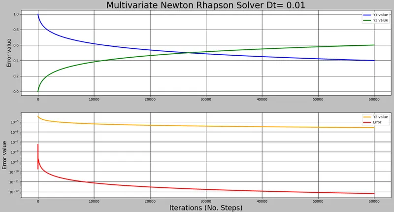
General results:
For a timestep of 1:

For a timestep of 0.1:

For a timestep of 0.01

Conclusion
The higher the time step the higher the time step given the greater the error will be, having visually the same y1, y2, y3 values, although the error increases proportional to the timestep.
Due to the constant final time of 10 minutes the change of timestep increases the computational time, being a directly proportional increase and number of steps calculated.
A step error is generated at the beginning of the calculations being wider when decreasing the timestep.
Due to the constant increase in the error vale of the Y3 result, for the 0.1 timestep calculation the ideal steps are 2686.5 steps resulting in 2e-10 general error value. Being constant in relationship to the visualization in the other results.
Reference