Week 6 - Data analysis

DATA SCIENCE CHALLENGE

Aim:

1. Use python programing to analyze the data provided with the challenge.
2. Plot the graph as per user inputs
3. Do a basic performance calculation for the IC engine with the available data set.

Problem Statement:

Data-science is a wide and new field in engineering and sciences. Data science gives us a vast set of data which needs to be studied for forecasting the future behavior of the data being studied. Thus, writing a program that can do the same with the set of data provided will be simplifying this process for the data scientists.

Theory:

Calculation of power output and Specific fuel consumption (SFC)

power_output = n*area*stroke_cycle/(1000)

where;

n= nu,ber of cylinders

area = area under PV diagram (obtained from data set)

stroke_cycle = revolutions per second/ 2

SFC = (fuel_consumption * 10⁶ * stroke_cycle * 3600) / (power_output * 1000)

Program:

import math
import matplotlib.pyplot as plt
import numpy as np
from scipy.integrate import simps

#Compatibility check
fname = input("Enter the filename:")

if fname == 'engine_data.out':
	print('file is valid')

else:
	print('file is invalid')
	exit()


def compatibility_check(a):
	if 'CONVERGE' not in a:
		print('Please provide converge output file to process')
		exit()
	else:
		print('Compatibility check is successful')
		pass

#try:
open('engine_data.out')


# Creating an empty array to store the values of Volume and pressure respectively
Volume = []
pressure = []

line_count = 1
for line in open('engine_data.out'):
	if '#' not in line:
		Volume.append(float(line.split()[7]))
		pressure.append(float(line.split()[1]))
	line_count = line_count + 1 



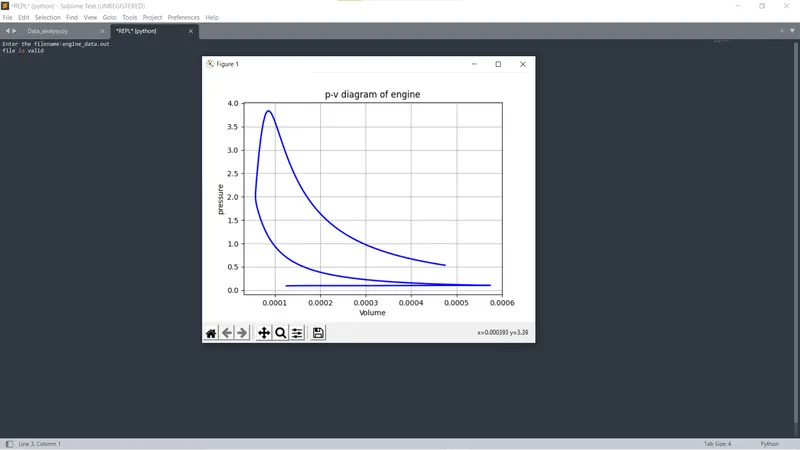
#plotting p-v diagram
plt.plot(Volume, pressure, linewidth = 2, color = 'b')
plt.xlabel('Volume')
plt.ylabel('pressure')
plt.title("p-v diagram of engine")
plt.grid()
plt.show()

area = float(simps(pressure,Volume))
print('Area under the curve using Simpsons Rule :' +str(area) + ' units')
print('Work done by the engine : ' + str(area) + ' MJ')
area = area * 1e6
print('Work done by engine : ' + str(area) + ' J')



# Inputs
# Speed of an Engine
rpm = 1500
rps = 1500/60
stroke_cycle = rps/2
# Fuel consumption in micrograms per 1 stroke cycle
fuel_consumption = 20
# Engine specifications
# Number of cylinder
n = 1
# 4 stroke engine
# Calculation of power output and Specific fuel consumption
power_output = n*area*stroke_cycle/(1000)
print('power output from engine : ' + str(power_output) + 'KW')
SFC = (fuel_consumption*pow(10,-6)*stroke_cycle*3600)/(power_output*1000)
print('Specific Fuel consumption, SFC = ' + str(SFC) + ' (kg/hr)/KW')
print('t')

# Calculation of Area under PV diagram
Area = np.trapz(pressure,Volume)
print('Area under curve using trapezoidal rule : ' + str(Area) + 'units')
print('Work done by the engine : ' + str(Area) + ' MJ' )
Area = Area * 1e6
print('Work done by engine : ' + str(Area) + ' J')
power_output = n*Area*stroke_cycle/(1000)
print('power output from the engine : ' + str(power_output) + 'KW')
SFC = (fuel_consumption*pow(10,-6)*stroke_cycle*3600)/(power_output*1000)
print('Specific Fuel consumption, SFC = ' + str(SFC) + ' (kg/hr)/KW')
print('t')

# Transposing columns in to row matrix and converting them in to float type from string type
#transpose = np.transpose(data)
#float_f = transpose.astype(np.float)

# Array for header and their units
#parameters = ['Crank','Pressure','Maximum Pressure','Minimum Pressure','Mean Temperature','MaximumTemperature','Minimum Temperature','Volume','Mass','Density','Integrated HR','HRrate','Cp','Cv','gamma','Kinematic Viscosity','Dynamic Viscosity']

units = ['(DEG)','(Mpa)','(Mpa)','(Mpa)','(K)','(K)','(K)','pow(m,3)','(kg)','(kg/(pow(m,3)))','(J)','(J)','(J/time)'
,'(J/kgK)','(J/kgK)','','pow(m,2)/s','(Ns/pow(m,2)']


# Providing user choice of picking 2 parameters for plotting

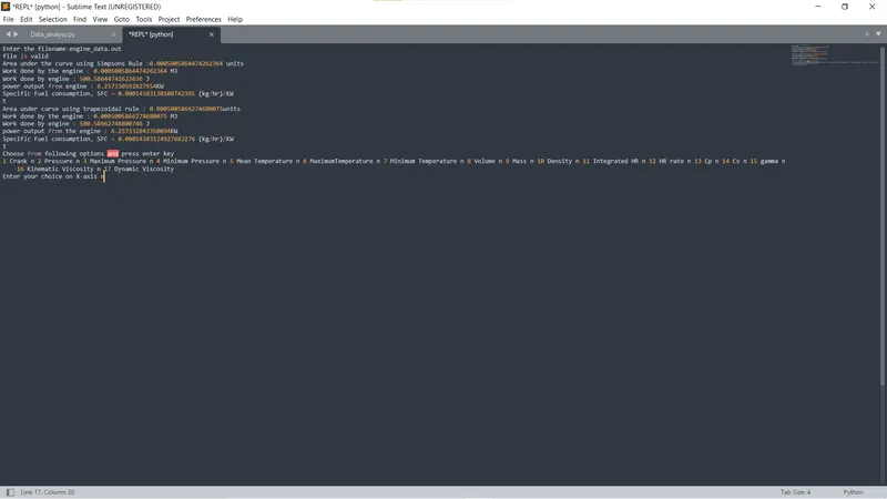
print('Choose from following options and press enter key')

print('1 Crank n 2 Pressure n 3 Maximum Pressure n 4 Minimum Pressure n 5 Mean Temperature n 6 MaximumTemperature n 7 Minimum Temperature n 8 Volume n 9 Mass n 10 Density n 11 Integrated HR n 12 HR rate n 13 Cp n 14 Cv n 15 gamma n 16 Kinematic Viscosity n 17 Dynamic Viscosity')

X = int(input('Enter your choice on X-axis n'))
Y = int(input('Enter your choice on Y-axis n'))
n = X-1
m = Y-1
crank = []
max_pressure = []
min_pressure = []
mean_temp = []
max_temp = []
min_temp = []
mass = []
density = []
integra_HR = []
HRrate = []
Cp = []
Cv = []
gamma = []
Kinematic_viscosity = []
Dynamic_viscosity = []


line_count = 1
for line in open('engine_data.out'):
	if '#' not in line:
		crank.append(float(line.split()[0]))
		max_pressure.append(float(line.split()[2]))
		min_pressure.append(float(line.split()[3]))
		mean_temp.append(float(line.split()[4]))
		max_temp.append(float(line.split()[5]))
		min_temp.append(float(line.split()[6]))
		mass.append(float(line.split()[8]))
		density.append(float(line.split()[9]))
		integra_HR.append(float(line.split()[10]))
		HRrate.append(float(line.split()[11]))
		Cp.append(float(line.split()[12]))
		Cv.append(float(line.split()[13]))
		gamma.append(float(line.split()[14]))
		Kinematic_viscosity.append(float(line.split()[15]))
		Dynamic_viscosity.append(float(line.split()[16]))
	line_count = line_count + 1 
parameter = np.array([crank,pressure,max_pressure,min_pressure,mean_temp,max_temp,min_temp,Volume,mass,density,integra_HR,HRrate,Cp,Cv,gamma,Kinematic_viscosity,Dynamic_viscosity])
parameters = ['Crank','Pressure','Maximum Pressure','Minimum Pressure','Mean Temperature','MaximumTemperature','Minimum Temperature','Volume','Mass','Density','Integrated HR','HRrate','Cp','Cv','gamma','Kinematic Viscosity','Dynamic Viscosity']
units = ['(DEG)','(Mpa)','(Mpa)','(Mpa)','(K)','(K)','(K)','pow(m,3)','(kg)','(kg/(pow(m,3)))','(J)','(J)','(J/time)'
,'(J/kgK)','(J/kgK)','','pow(m,2)/s','(Ns/pow(m,2)']



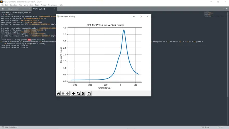
plt.figure("User input plotting")
plt.plot(parameter[n],parameter[m],linewidth=3)
plt.title(' plot for ' + parameters[m]+ ' versus ' +parameters[n],color='k')
plt.xlabel(parameters[n] + ' ' +units[n])
plt.ylabel(parameters[m] + ' ' +units[m])
plt.grid()
plt.show()

Results:

program screenshots

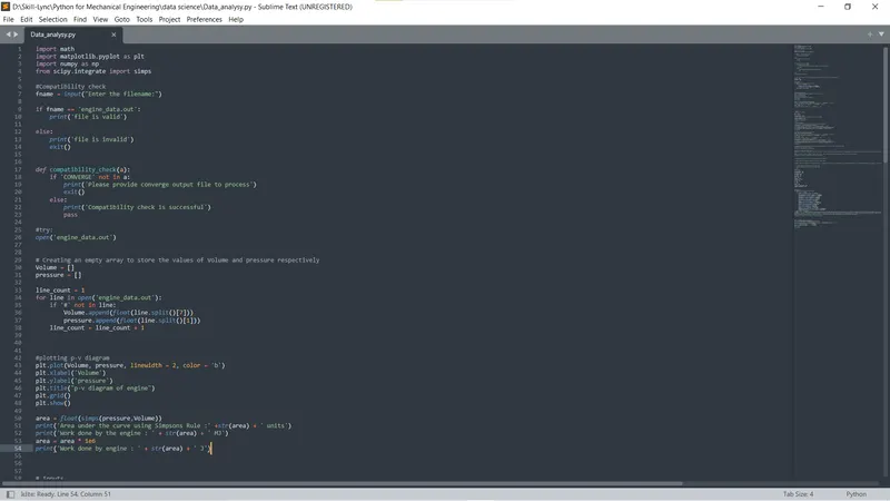
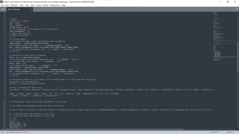
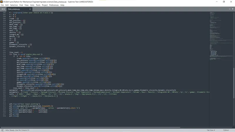
step-by-step for result

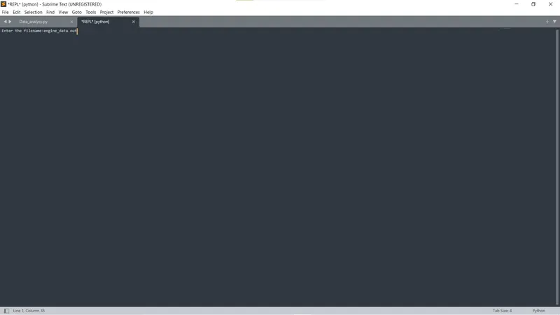
Area under the curve using Simpsons Rule :0.0005005864474262364 units
Work done by the engine : 0.0005005864474262364 MJ
Work done by engine : 500.58644742623636 J
power output from engine : 6.257330592827954KW
Specific Fuel consumption, SFC = 0.00014383130100742395 (kg/hr)/KW

Area under curve using trapezoidal rule : 0.0005005866274680075units
Work done by the engine : 0.0005005866274680075 MJ
Work done by engine : 500.58662746800746 J
power output from the engine : 6.257332843350094KW
Specific Fuel consumption, SFC = 0.00014383124927683276 (kg/hr)/KW