Week 6 - Data analysis

**Data analysis**

AIM:

To perform a Data analysis on Engine Parameters using python code

Objective :

To write a python code that does the following things :

1. Data visualizing
2. Compatability check
3. basic performance calculation

Python code :

"""
# Data Analysis on Engine
"""

# importing essential library tools
import math # importing math library tools
import matplotlib.pyplot as plt # importing plotting library tools
import numpy as np # importing numberical and logical libraty tools
from scipy.integrate import simps, trapz as trapz # importing the simpson rule and trapezoidal rule library tools

# file input
file='engine_data.out' # inputing the data file

# compatability check
try:
file=open('engine_data.out')
line_count=1
except:
print('file not recognized. please provide a valid converge output file')

# Values storage
volume=[] # storing the values of volume in an array
pressure=[] # storing the values of pressure in an array

# pressure and volume in the data file
v=2 # volume
p=8 # pressure

# array storing
data=[] # array stored in data form

for line in open('engine_data.out'): # openning the file
if '#' not in line: # excluding the lines which start with pound
data.append(line.split()) # attaching the stored data to the loop
if line_count >=6: # creating the line count in loop
volume.append(float(line.split()[v-1])) # attaching the volume to the loop
pressure.append(float(line.split()[p-1])) # attaching the pressure to the loop
line_count=line_count+1 # incrementing the line count

# plotting for PV diagram
plt.figure(1)
plt.plot(pressure,volume,color='r')
plt.grid()
plt.xlabel('Pressure in MPa')
plt.ylabel('Volume in m^3')
plt.title('P-V diagram of Engine')
plt.show()

# Computation of area under p-v diagram
area=simps(pressure,volume) # using simpson rule
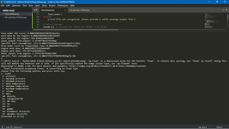
print('Area under the curve:'+str(area)+'units')
print('work done by the engine:'+str(area)+'MJ')
area=area*1e6
print('work done by the engine:'+str(area)+'J')

# input parameters
rpm=1500 # Engine speed in rpm
rps=1500/60 # Engine speed in seconds
stroke_cycle=rps/2 # stroke cycle

# fuel consumption in mcg/strokecycle
fuel_consumption=20

# Engine specification
n=1 # no of cyclinder in 4 stroke engine

# Computation of power output and specific fuel consumption
power_output=n*area*stroke_cycle/1000
print('power_output from engine:'+str(power_output)+'kW')
sfc=(fuel_consumption*pow(10,-6)*stroke_cycle*3600)/(power_output*1000)
print('specific fuel consumption, sfc='+str(sfc)+'(kg/hr)/(kW)')

# Computation of area under PV diagram
Area=np.trapz(pressure,volume) # trapezoidal rule
print('Area under curve by trapexoidal rule:'+str(Area)+'units')
print('Engine work done:'+str(Area)+'MJ')
Area=Area*1e6
print('Engine work done:'+str(Area)+'J')
power_output=n*Area*stroke_cycle/1000
print('Power output from engine:'+str(power_output)+'kW')
sfc=fuel_consumption*pow(10,-6)*(stroke_cycle*3600)/(power_output*1000)
print('specific fuel consumption, sfc:'+str(sfc)+'kg/hr/kW')
print('t')

transpose=np.transpose(data) # transposing columns into row matrix
float_f=transpose.astype(np.float) # converting to float type

# header and thier inits
parameters=['crank','pressure','max.pressure','min.pressure','mean.temperature','max.temperature','min.temperature','volume','mass','density','integrated HR','HR rate','Cp','Cv','Gamma','Kin.Viscocity','Dyn.Viscocity']
units=['deg','MPa','MPa','MPa','K','K','K','M^3','kg','kg/m3','J','J/time','J/kgK','J/kgK','m2/s','Ns/m2']

print('choose from the following options and press enter key')
print('1- crank \n 2- pressure \n 3- maximum pressure \n 4- minimum pressure \n 5- mean temperature \n 6- maximum temperature \n 7- minimum temperature \n 8- volume \n 9- mass \n 10- density \n 11- integrated HR \n 12- HR rate \n 13- Cp \n 14- Cv \n 15- gamma \n 16- kinematic Viscocity \n 17- dynamic Viscocity')

# X=int(input('Enter your choices on x-axis:'))
# Y=int(input('Enter your choices on y-axis:'))
X = 1
Y = 2

# X = 1
# Y = 4

plt.figure(2)
plt.plot(float_f[X-1],float_f[Y-1],color='blue')
plt.title('plot for' + parameters[X-1]+ 'vs'+ parameters[Y-1] ,color='blue')
plt.xlabel(parameters[X-1]+''+units[X-1])
plt.ylabel(parameters[Y-1]+''+units[Y-1])
plt.grid()
plt.show()

EXPLANATION :

• Step 1 : importing required library tools.
  
  • importing the required modules tools like math, matplotlib.pyplot, numpy and scipy.integrate.
  • from scipy library importing simps and trapz library tools.
• Step 2: Input parameters.
  
  • inputing the given data from the objective which need to be analysed and checked.
  • try command helps in checking the compatibility of the file.
  • the file which is not recognized need to prove a converge output file.
• Step 3: Computation
  
  • creating null array for pressure and volume.
  • plotting the pv diagram from a data file which is in line 2 and 8 respecitively.
  • for calculating the area under PV diagram we use simpson rule and calculating popt and sfc we will be using the input parameters.
  • repeating the same proccess but now we will be using trapezoidal rule and doing the same for popt and sfc.
  • Transposing the columns in row matrox and converting into float type and plotting it.
• Step 4: plotting
  
  • initially we will be creating the array for header and thier units i.e. parameters and units,
  • then providing user the choice of picking using two parameters for plotting.
  • in python the minimum value starts from 0.
  • then desired graph will be plotted as per the user.

Output :

Figure 1 :

P-V diagram of Engine

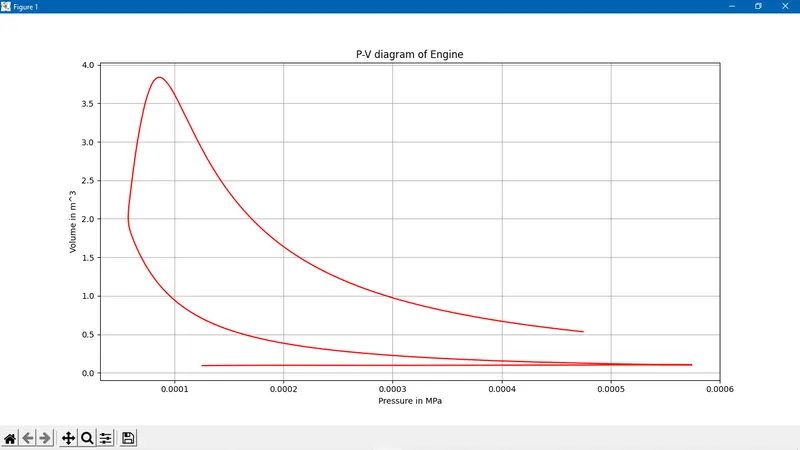
Figure 2 :

X = 1
Y = 2

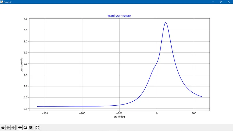
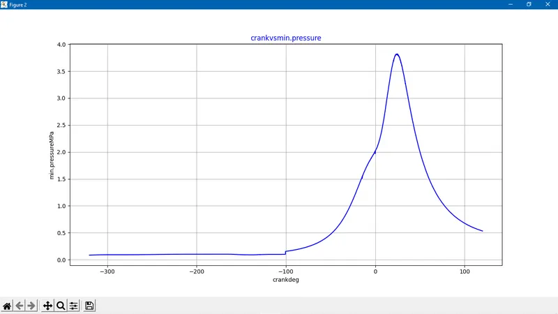
Figure 3 :

X = 1
Y = 4

Output Of the code :