Rankine cycle Simulator

AIM :- To create rankine cycle simulation using MATLAB

Objective :-

To Calculate

• Net work output
• Back work ratio
• plot T-s(Temperature vs. specific entropy) and h-s(An enthalpy–entropy) plots for the given set of inputs.

• Net work output

From the output work subtraction to the input work is called the Net work output.

Wnet = Wout - Win

• Back work ratio

The ratio of the pump work to the turbine work is called the back-work ratio.

BW = Wp/Wt

• Entropy

Heat flow over the temp. (dQ/T)

• Enthalpy

The sum of the internal energy(E) added to the product of the pressure(P) and volume(V) of the system.

H = E + PV or d H = T d S + P d V

Some inputs value (Given Data):-

Turbine Inlet temperature = 400° C

Turbine Inlet Pressure = 30 bars

Turbine Outlet Pressure = 0.05 bars = Condenser Inlet Pressure

Solution :-

• Some Basic Formula

Boiler h2 + qH = h3 ⇒ qH = h3 − h2 (in)
Turbine h3 = h4 + wT ⇒ wT = h3 − h4 (out)
Condenser h4 = h1 + qL ⇒ qL = h4 − h1 (out)
Pump h1 + wP = h2 ⇒ wP = h2 − h1 (in)

• Process of Rankine Cycle
• Process 1–2: The working fluid is pumped from low to high pressure. As the fluid is a liquid at this stage, the pump requires little input energy.

Process 1-2 = Isentropic compression ,

• Process 2–3: The high-pressure liquid enters a boiler, where it is heated at constant pressure by an external heat source to become a dry saturated vapour. The input energy required can be easily calculated graphically, using an enthalpy–entropy chart (h–s chart, or Mollier diagram), or numerically, using steam tables or software.

Process 2-3 = Constant pressure heat addition in boiler ,

• Process 3–4: The dry saturated vapour expands through a turbine, generating power. This decreases the temperature and pressure of the vapour, and some condensation may occur. The output in this process can be easily calculated using the chart or tables noted above.

Process 3-4 = Isentropic expansion ,

• Process 4–1: The wet vapour then enters a condenser, where it is condensed at a constant pressure to become a saturated liquid.

Process 4-1 = Constant pressure heat rejection in condenser ,

If a water exists as a liquid at the saturation temperature and pressure with quality of x = 0, it is called a saturated liquid state (single-phase).

The vapor quality is equal to 1, it is referred to as the saturated vapor state or dry steam (single-phase).

Between these two states, we talk about vapor-liquid mixture or wet steam (two-phase mixture). At constant pressure, an addition of energy does not changes the temperature of the mixture, but the vapor quality and specific volume changes.

--------------------------------------------CODE-------------------------------------------------------------

clear all
close all
clc

P1 = input('Enter the pressure in the boiler (bar): ') % Turbine Inlet Pressure = 30 bars
P2 = input( 'Enter the pressure in the condenser (bar): ' ) % Turbine Outlet Pressure = 0.05 bars
T1 = input( 'Enter the temperature at the turbine inlet (deg-C) : ' ) % Turbine Inlet temperature = 400° C

if P1 >200
fprintf('n Pressure value entered is out of range...nPrograms Exits...n');
return;
end
if T1 > 1999
fprintf('n Temperature is out of range...nProgram exits..n');
return;
end
if T1 < XSteam('Tsat_p',P1)
fprintf('n Temperature is out of range...nProgram exits..n');
return;
end
if P2 > P1
fprintf('n Invalid input parameters...Condenser pressure cannot be higher than boiler pressure...n Program exits...n');
return;
end

P1 = 30 % Boiler Outlet Pressure = 30 bars = Turbine Inlet Pressure
P2 = 0.05 % Turbine Outlet Pressure = 0.05 bars = Condenser Inlet Pressure
P3 = P2 % Condenser Outlet Pressure = Pump Inlet Pressure % Isoboric Process
P4 = P1 % Pump Outlet Pressure = Boiler Inlet Pressure % Isoboric Process

% Turbine Inlet
T1 = 400 % Turbine Inlet temperature = 400° C
S1 = XSteam('s_pT' , P1,T1) % specific entropy as function of presser and temperature
H1 = XSteam('h_pT' , P1,T1) % specific enthalpy as function of presser and temperature

% Condenser Inlet
S2 = S1 % isentopic expansion - Entropy remain same
T2 = XSteam('T_ps' , P2,S2) % Temprature as function of presser and entropy
H2 = XSteam('h_ps', P2,S2) % specific enthalpy as function of presser and entropy

% Pump Inlet
T3 = XSteam('Tsat_p' ,P3) % Temperature_condenser_sat
S3 = XSteam('sL_T',T3) % Saturated liquid entropy
H3 = XSteam('hL_T',T3) % Saturated liquid enthalpy

% Boiler Inlet
S4 = S3; % Isentropic Process
T4 = XSteam('T_ps' ,P4,S4) % Temprature as function of presser and entropy
H4 = XSteam('h_ps',P4,S4) % specific enthalpy as function of presser and entropy

S5 = XSteam('sL_p',P4) % Saturated liquid entropy
S6 = XSteam('sV_p',P4) % Saturated Volume entropy
H5 = XSteam('hL_p',P4) % Saturated liquid enthalpy
H6 = XSteam('hV_p',P4) % Saturated Volume enthalpy

T5 = XSteam('Tsat_p' ,P1) % Saturated Temprature
T6 = T5 % Temprature remain same

W_P = H4 - H3 % Work Done on Pump
Q_add = H1 - H4 % Hear Addition in Boiler
W_T = H1 - H2 % Work Done by Turbine
Q_re = H2 - H3 % Hear Rejection by Condenser
W_net = W_T - W_P % Net work output
n_th = W_net/Q_add % Thermal efficiency

BW = W_P/W_T % Back work ratio

subplot(2,1,1)

temperature_range = linspace(10,400,100);
for i=1: length(temperature_range)
entropy_range_lower(i) = XSteam('sL_T',temperature_range(i));
entropy_range_upper(i) = XSteam('sV_T',temperature_range(i));
enthalpy_range_lower(i) = XSteam('hL_T',temperature_range(i));
enthalpy_range_upper(i) = XSteam('hV_T',temperature_range(i));
end

plot([S1 S2],[T1 T2],'color','yellow','linewidth',2,'marker','O','displayName','Turbine')
hold on
plot( [S2 S3],[T2 T3],'color','blue','linewidth',2,'marker','O','displayName','Condenser')
hold on
plot( [S3 S4],[T3 T4],'color','green','linewidth',2,'marker','O','displayName','Pump')
hold on
plot( [S4 S5],[T4 T5],'color','cyan','linewidth',2,'marker','O','displayName','Pre-heater')
hold on
plot( [S5 S6],[T5 T6],'color','red','linewidth',2,'marker','O','displayName','Boiler')
hold on
plot( [S6 S1], [T6 T1],'color','magenta','linewidth',2 ,'marker','O','displayName','Super-heater')
hold on
plot(entropy_range_lower,temperature_range,'color','black','linewidth',1,'displayName','Saturation line');
hold on;
plot(entropy_range_upper, temperature_range,'color','black','linewidth',1,'displayName','Saturation line');
hold on;
title('S vs T')
axis([0 8 0 750])
xlabel('Specific entropy kJkgK')
ylabel('Temperature ^0C')
legend

subplot(2,1,2)

plot( [S1 S2],[H1 H2],'color','m','linewidth',2,'marker','O')
hold on
plot( [S2 S3],[H2 H3],'color','b','linewidth',2,'marker','O')
hold on
plot([S3 S4],[H3 H4],'color','y','linewidth',2,'marker','O')
hold on;
plot( [S4 S5],[H4 H5],'color','g','linewidth',2 ,'marker','O')
hold on
plot( [S5 S6],[H5 H6],'color','b','linewidth',2 ,'marker','O')
hold on
plot( [S6 S1],[H6 H1],'color','g','linewidth',2 ,'marker','O')
hold on
plot(entropy_range_lower,enthalpy_range_lower,'color','r','linewidth',1);
hold on;
plot(entropy_range_upper, enthalpy_range_upper,'color','r','linewidth',1);
hold on;
title('H vs S')
axis([0 8 0 3500])
ylabel('Specific entropy kJkgK')
xlabel('Specific enthalpy kjkg')
legend ('Turbine','Condenser','Pump' ,'Boiler')

------------------------------RESULT---------------------------

• Net work output = 1.1179e+03
• Back work ratio = 0.0027
• Thermal Efficiency = 36.17%

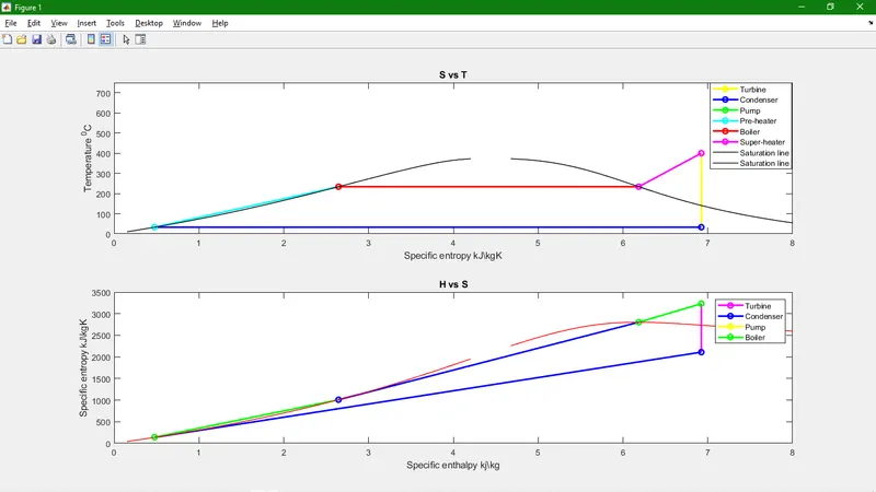
------------------------------Conclusion-----------------------

Here, Temperature is directly affected to entropy.