Data Analysis Using Python

Data Analysis

Data analysis is a process of inspecting, cleansing, transforming, and modelling data with the goal of discovering useful information, informing conclusions, and supporting decision-making. Data analysis has multiple facets and approaches, encompassing diverse techniques under a variety of names, and is used in different business, science, and social science domains. Data analysis plays a role in making decisions more scientific and helping businesses operate more effectively.

Data Analysis can be separated and organized into 6 types:-
1. Descriptive Analysis
2. Exploratory Analysis
3. Inferential Analysis
4. Predictive Analysis
5. Causal Analysis
6. Mechanistic Analysis

1. Descriptive Analysis

Goal - Describe or Summarize a set of Data

Description - The very first analysis performed. It generates simple summaries about samples and measurements, common descriptive statistics (measures of central tendency, variability, frequency, position, etc).

Example - Take the COVID-19 statistics page on google, for example, the line graph is just a pure summary of the cases/deaths, a presentation and a description of the population of a particular country infected by the virus.

Summary - Descriptive Analysis is the first step in analysis where you summarize and describe the data you have using descriptive statistics, and its result is a simple presentation of your data.

2. Exploratory Analysis (EDA)

Goal - Examine or explore data and find relationships between variables that were previously unknown.

Description - EDA helps you discover relationships between measures in your data, which do not evidence for the existence of the correlation, as denoted by the phrase (Correlation doesn’t imply causation). Useful for discovering new connections — forming hypotheses and drives design planning and data collection.

Example - Climate change is an increasingly important topic as the global temperature is gradually rising over the years. One example of EDA on climate change is by taking the rise in temperature over the years, say 1950 to 2020 for example, and the increase of human activities and industrialization, and form relationships from the data, e.g. increasing number of factories, cars on the road and aeroplane flights increase correlates.

Summary - EDA explores data to find relationships between measures that tell us they exist, without the cause. They can be used to formulate hypotheses.

3. Inferential Analysis

Goal - Using a small sample of data to infer about a larger population. The goal of statistical modelling itself is all about using a small amount of information to extrapolate and generalize information to a larger group.

Description - Using estimated data that value in population and give a measure of uncertainty (standard deviation) in your estimation. Accuracy of inference depends heavily on the sampling scheme; if the sample isn’t representative of the population, the generalization will be inaccurate (refer to Central Limit Theorem)

Example - The idea of inferring about the population at large with a smaller sample is quite intuitive, many statistics you see on the media and the internet are inferential, a prediction of an event based on a small sample. To give an example, a psychology study for the benefits of sleep, a total of 500 people were involved in the study, when followed up with the candidates, they reported having better overall attention and well-being with 7–9 hours of sleep, while those with less sleep and more sleep suffered from reduced attention and energy. This report from 500 people was just a tiny portion of 7b people in the world, thus an inference of the larger population.

Summary - IA extrapolates and generalizes the information of the larger group with a smaller sample to generate analysis and predictions.

4. Predictive Analysis

Goal - Using historical or current data to find patterns to make predictions about the future

Description - The accuracy of the predictions depends on the input variables. Accuracy also depends on the types of models, a linear model might work well in some cases, and vice-versa. Using a variable to predict another doesn’t denote causal relationships.

Example - The 2020 US election is a popular topic and many prediction models are built to predict the winning candidate FiveThirtyEight did a great 2016 Election forecast and is back at it again in 2020. Prediction analysis for an election would require input variables such as historical polling data, trends and the current polling data in order to get a good prediction. Something as large as an election wouldn’t just be using a linear model, but a complex model with certain tunings to best serve its purpose.

Summary - PA takes data from the past and present to make predictions about the future.

5. Causal Analysis

Goal - Looks at the cause and effect of relationships between variables, focused on finding the cause of a correlation.

Description - To find the cause, you have to question whether the observed correlations driving your conclusion are valid, as just looking at the data (surface) won’t help you discover the hidden mechanisms underlying the correlations. Applied in randomized studies focused on identifying causation. The gold standard in data analysis, scientific studies where the cause of the phenomenon is to be extracted and singled out, like separating the wheat from the chaff

Challenges - Good data is hard to find and requires expensive research and studies. These studies are analyzed in aggregate (multiple groups), and the observed relationships are just average effects (mean) of the whole population (meaning the results might not apply to everyone)

Example - Say you want to test out this new drug that improves human strength and focus, and to do that you perform randomized control trials for the drug to test the effect of the drug. You compare the sample of candidates for your new drug vs the candidates receiving mock control with a few tests for strength and overall focus and attention and observe how the drug affects the outcome

Summary - CA is about finding out the causal relationship between variables, change one variable and what happens to another.

6. Mechanistic Analysis

Goal - Understand exact changes in variables that lead to other changes in other variables

Description - Applied in physical or engineering sciences, situations that require high precision and little room for error(only noise in data is measurement error). Designed to understand a biological or behavioural process, the pathophysiology of a disease, or the mechanism of action of an intervention. (by NIH)

Example - Many graduate-level research and complex topics are suitable examples, but to put it in a simple manner, let’s say an experiment is done to simulate safe and effective nuclear fusion to power the world, mechanistic analysis of the study would entail a precise balance of controlling and manipulating variables with highly accurate measures of both variables and the desired outcomes. It’s this intricate and meticulous modus operandi (strategy) towards these big topics that allows for scientific breakthroughs and the advancement of society.

Summary - MA is in some ways a predictive analysis, but modified to tackle studies that require high precision and meticulous methodologies for physical or engineering science. Summary

Compatibility Check

The compatibility check confirms the file name and the file type before executing. It takes the input as file name from the user and validates the converge file for which data analysis is being carried out and if the file is not valid the program stops execution.

#File Compatibility Check

#Enter the File Name
file_name=input("Enter file name with extension:")

try:
	data = open(file_name,'r')
	print("nFile is compatible")

except FileNotFoundError:
	print('"File not recognized. Please provide a valid CONVERGE output file"')
	exit()

Output

Enter file name with extension:engine_data.out

File is compatible

Basic Performance Calculation

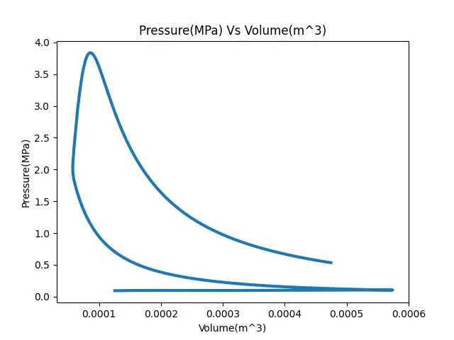
Workdone=Pressure*Volume= Area under the PV Curve.

The area under the PV curve is found using the NumPy trapz function.

Power can be defined as the rate of doing work. We have work done for one complete cycle using the rpm of the engine we can find the number of revolutions per second hence find the rate of doing work which is termed as power.

Specific fuel consumption is defined as the amount of fuel consumed divided by the brake horsepower.

#Area under the p-v diagram
print("nBasic Calcuations")
pressure=[]
volume=[]
for data in open(file_name):
	if '#' not in data:
		volume.append(float(data.split()[7]))
		pressure.append(float(data.split()[1]))

area= np.trapz(pressure,volume)*pow(10,6)

#Power output of the engine
rpm = 1500
power = area*(rpm/60)

#Specific fuel consumption
f_mass = 20*pow(10,-6)
sfc=f_mass/power

Output

Basic Calcuations
The area under the P-V diagram is 500.59
The the power output of this engine is 12514.67
The specific fuel consumption is 1.6e-09

Taking input from the user as column numbers to plot the respective graph

To display the data available in the first five lines of the file we extract the column names with their respective units and store them in the form of a list and print it to show the available data.

#Displaying the File Data
c_no=[]
c_name=[]
c_unit=[]

ct=1

for data in open(file_name):
	if ct==2:
		temp=data.split()
		for i in range (2,len(temp)):
			c_no.append(temp[i])
	if ct==3:
		temp=data.split()
		for i in range (1,len(temp)):
			c_name.append(temp[i])
	if ct==4:
		temp=data.split()
		for i in range (1,len(temp)):
			c_unit.append(temp[i])

	if ct==5:
		print("nFollowing data is available")
		for i in range(0,len(c_no)):
			print(c_no[i],c_name[i],c_unit[i])
	ct=ct+1

After printing the data it takes input from the user for the x-axis and y-axis data in the form of the serial numbers. The serial number is then used to extract the respective data from the file, it acts to provide the column identification whose data is extracted.

The given input also acts as the index for the column name and unit which is used to label the plot and save the figure.

#Taking input for data display from user
x_axis=int(input("nSelect X-axis data as per Serial Number:"))-1
y_axis=int(input("nSelect Y-axis data as per Serial Number:"))-1
data_x=[]
data_y=[]

for data in open(file_name):
	if '#' not in data:
		data_x.append(float(data.split()[x_axis]))
		data_y.append(float(data.split()[y_axis]))

#Plot
plt.plot(data_x,data_y,linewidth=3)
plt.xlabel(c_name[x_axis]+c_unit[x_axis])
plt.ylabel(c_name[y_axis]+c_unit[y_axis])
plt.title(c_name[y_axis]+c_unit[y_axis]+" Vs "+c_name[x_axis]+c_unit[x_axis])
plt.savefig(c_name[y_axis]+c_unit[y_axis]+"Vs"+c_name[x_axis]+c_unit[x_axis]+".png")
plt.show()

Output

Enter file name with extension:engine_data.out

File is compatible

Basic Calcuations
The area under the P-V diagram is 500.59
The the power output of this engine is 12514.67
The specific fuel consumption is 1.6e-09

Following data is available
1 Crank (DEG)
2 Pressure (MPa)
3 Max_Pres (MPa)
4 Min_Pres (MPa)
5 Mean_Temp (K)
6 Max_Temp (K)
7 Min_Temp (K)
8 Volume (m^3)
9 Mass (kg)
10 Density (kg/m^3)
11 Integrated_HR (J)
12 HR_Rate (J/time)
13 C_p (J/kg-K)
14 C_v (J/kg-K)
15 Gamma (none)
16 Kin_Visc (m^2/s)
17 Dyn_Visc (N*s/m^2)

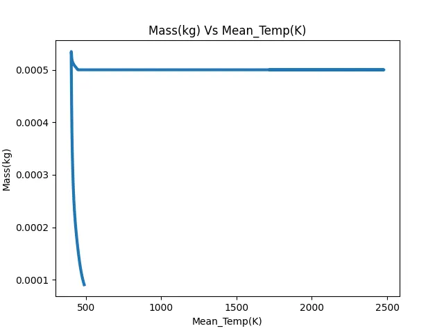
Select X-axis data as per Serial Number:5

Select Y-axis data as per Serial Number:9
>>> 

Mass vs Mean Temp

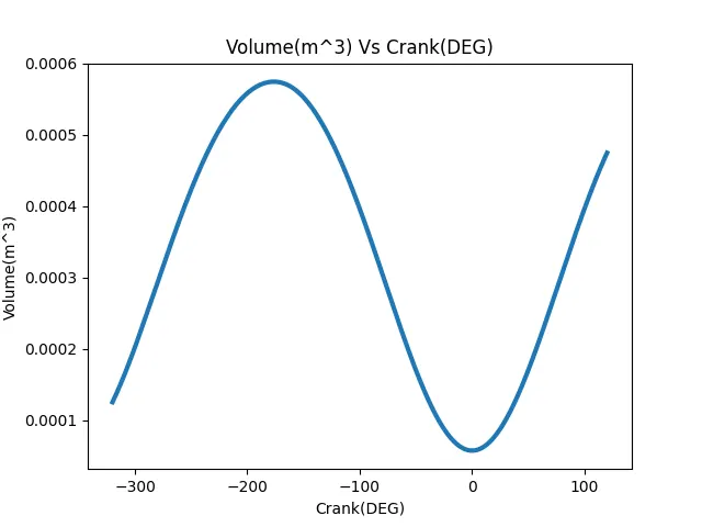
Volume vs Crank Angle

Pressure vs Volume

Complete Program

#Data Analysis
import numpy as np
import matplotlib.pyplot as plt
import math


#File Compatibility Check

#Enter the File Name
file_name=input("Enter file name with extension:")

try:
	data = open(file_name,'r')
	print("nFile is compatible")

except FileNotFoundError:
	print('"File not recognized. Please provide a valid CONVERGE output file"')
	exit()

#Area under the p-v diagram
print("nBasic Calcuations")
pressure=[]
volume=[]
for data in open(file_name):
	if '#' not in data:
		volume.append(float(data.split()[7]))
		pressure.append(float(data.split()[1]))

area= np.trapz(pressure,volume)*pow(10,6)

#Power output of the engine
rpm = 1500
power = area*(rpm/60)

#Specific fuel consumption
f_mass = 20*pow(10,-6)
sfc=f_mass/power

print("The area under the P-V diagram is",("{:.2f}".format(area)))
print("The the power output of this engine is",("{:.2f}".format(power)))
print("The specific fuel consumption is",(round(sfc,9)))

#Displaying the File Data
c_no=[]
c_name=[]
c_unit=[]

ct=1

for data in open(file_name):
	if ct==2:
		temp=data.split()
		for i in range (2,len(temp)):
			c_no.append(temp[i])
	if ct==3:
		temp=data.split()
		for i in range (1,len(temp)):
			c_name.append(temp[i])
	if ct==4:
		temp=data.split()
		for i in range (1,len(temp)):
			c_unit.append(temp[i])

	if ct==5:
		print("nFollowing data is available")
		for i in range(0,len(c_no)):
			print(c_no[i],c_name[i],c_unit[i])
	ct=ct+1

#Taking input for data display from user
x_axis=int(input("nSelect X-axis data as per Serial Number:"))-1
y_axis=int(input("nSelect Y-axis data as per Serial Number:"))-1
data_x=[]
data_y=[]

for data in open(file_name):
	if '#' not in data:
		data_x.append(float(data.split()[x_axis]))
		data_y.append(float(data.split()[y_axis]))

#Plot
plt.plot(data_x,data_y,linewidth=3)
plt.xlabel(c_name[x_axis]+c_unit[x_axis])
plt.ylabel(c_name[y_axis]+c_unit[y_axis])
plt.title(c_name[y_axis]+c_unit[y_axis]+" Vs "+c_name[x_axis]+c_unit[x_axis])
plt.savefig(c_name[y_axis]+c_unit[y_axis]+"Vs"+c_name[x_axis]+c_unit[x_axis]+".png")
plt.show()