Week 6: Conjugate Heat Transfer Simulation

Objectives:

1. Grid dependence test as the primary objective starting with an initial base grid

To run grid dependence test on 3 grid size and show that the outlet temperature converges to a particular value.

• Effect of supercycle stage interval

2. Supercyle stage interval is set to 0.01,0.02 and 0.03

For these three run, comparison of the total simulation time against the baseline configuration

Additional 3D outputs

• Addition of Y+ to the post.in file

Introduction

Conjugate heat transfer corresponds with the combination of heat transfer in solids and in fluids. In solids, conduction often dominates whereas in fluids, convection usually dominates. Efficiently combining heat transfer in fluids and solids is the key factor in designing effective coolers, heaters, or heat exchangers, no of fins required etc.. Forced convection is the most common way to achieve high heat transfer rate. In some applications, the performances are further improved by combining convection with phase change like boiling and condensation. CHT analysis is a prime importance where there is any form of heat transfer. For example the exhaust port of the IC engine, Graphic card simulation. A CHT flow simulation through a pipe is done in this project using Converge CFD software . Converge package has an extra advantage of Supercycling a CHT simulation and its effect is studied under this project. The postprocessing is done with Paraview .

 Super-cylcing in Converge : Super-cycling is used as a time control process. It uses clever averaging techniques to reach convergence quickly. Main poblem in CHT analyusis where both solid(Y+) and liquid regions are involved, is that both solvers cannot run at the same speed since solving in fluid domain is much faster because of the time scale difference for heat transfer in liquids as compared to the solids. This causes problems during the solution given that the solid side solver would not have reached a steady state/convergene in the time the liquid solver does. This is where the concept of super cycling is based.

 The steps it follows :

1. Solves the fluid and solid regions together with the transient solver during initial time steps.
2. Stores the instantaneous heat transfer coefficients value on the Interface boundary regions during this process.
3. Following that, it freezes the Fluid solver (Transient) and Time-averages the HTC and temperature values which is then applied as B.C at the interface.
4. Then it solves for the solid region temperature until it reaches steady state using steady state solver.
5. Then it updates the solid region temperature and unfreezes the Fluid solver (transient) and repeats this process until solid temperature converges.

An interface boundary separates two different materials or phases. In converge CHT simulations at least one such interface is required as a B.C.

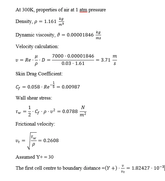
 At 300K, properties of air at 1 atm pressure

Geometry in Converge Studio :

Inner circle diameter 0.03 m and thickness 0.01m, the length of the cylinder is 0.2 m. After this boundary is flagged as per Boundary conditions.

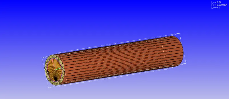
A diagnosis check is performed to check for errors.

Mesh:

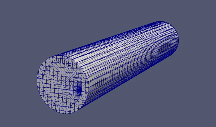
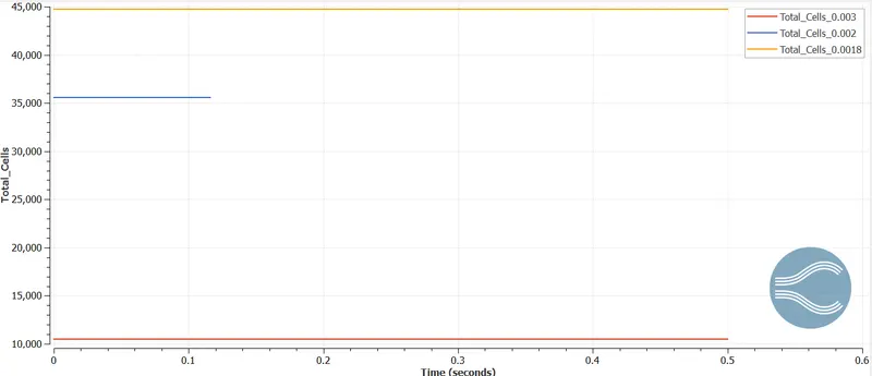
Case 1,2 and 3 respectively are Grid size- 0.03m;Grid size-0.02m;Grid size- 0.018m

Total cells

Case Setup

Case-setup In order to begin the case-setup, Time based simulation is turned on.

In Materials Air is selected to the predefined mixtures. Also solid simulation and species are also enabled.

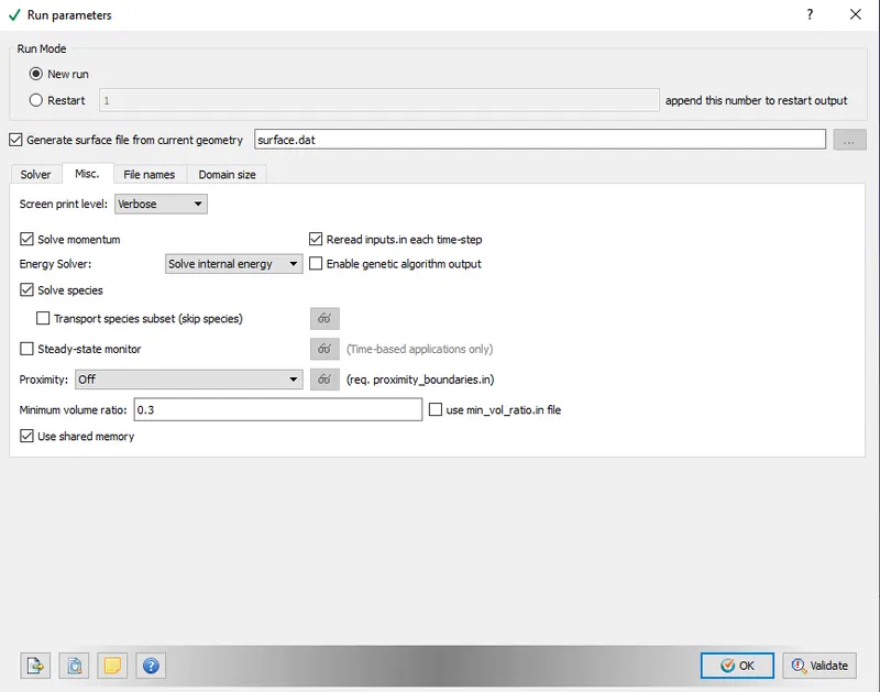
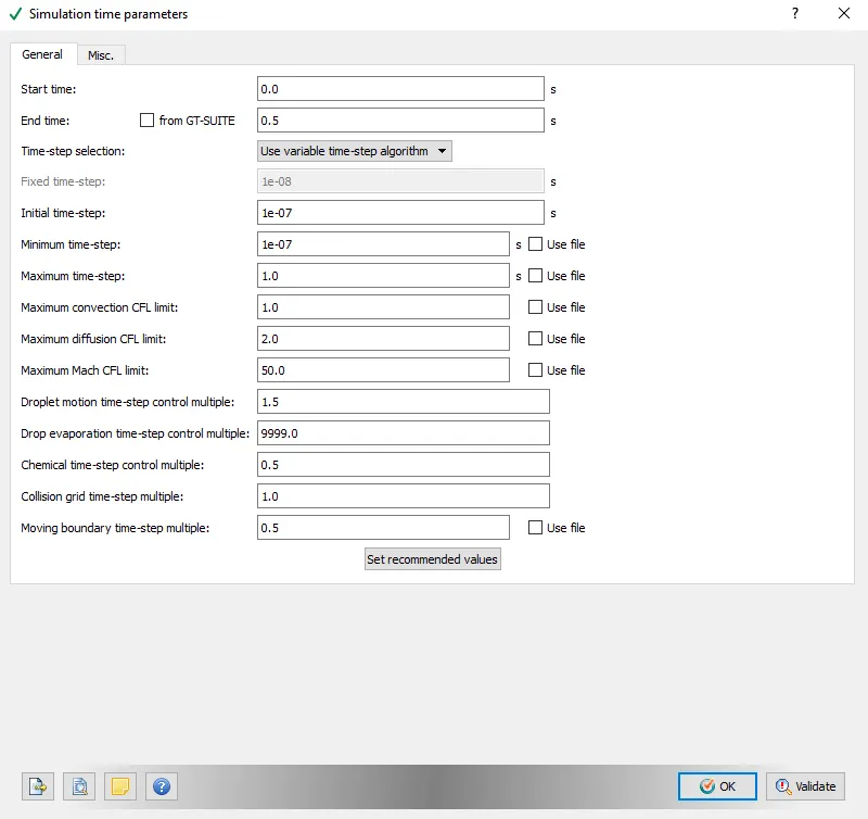
Then Gas simulation is opened with Global transport parameters with default settings. Then species tab is opened, in the Query available Aluminum as a solid species is chosen. Then for gas from the Query available list, N2 and O2 are chosen as a gas species. For, run Parameter under the Simulation Parameter the transient solver is chosen under the solver tab and then the Full Hydrodynmic is chosen under the simulation mode. And then the Compressible fluid flow is chosen under the Gas flow solver. In the simulation time parameter following changes are done.

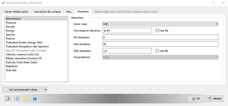
 In the solver time parameter, we only choose the pressure based solver and retain the remaining setting.

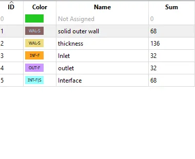
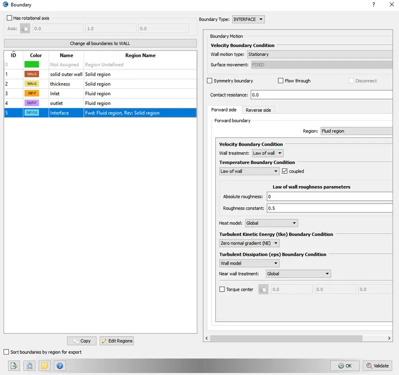
 The boundaries are added by clicking create multiple boundaries to create all boundaries at a once and name them like Outer_solid_wall, Solid_wall, inlet, outlet and interface.

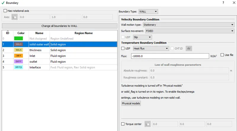
In the outer solid wall, boundary type selected is  wall. And -10000  is assigned to a Heat flux in the temperature boundary condition. The region is solid.

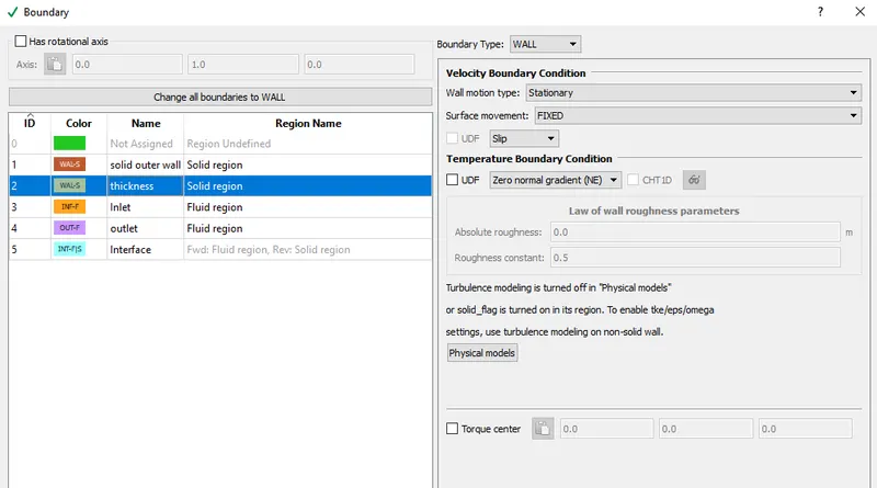
In the solid wall, the Wall type boundary condition is chosen. The velocity boundary condition is chosen as a slip and temperature boundary condition as a zero normal gradient. The region is a solid region.

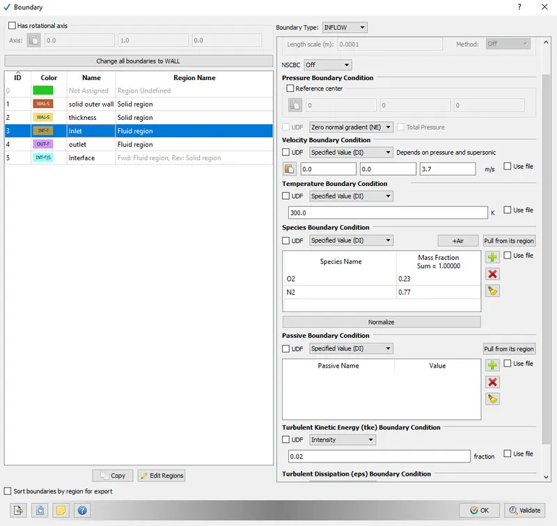
 For boundary type inflow: select the region as a Fluid region. The zero normal gradient is chiosen in the pressure boundary condition. In the velocity boundary condition 3.71 m/s is assigned in the z-positive direction. And 300K in the temperature boundary condition.

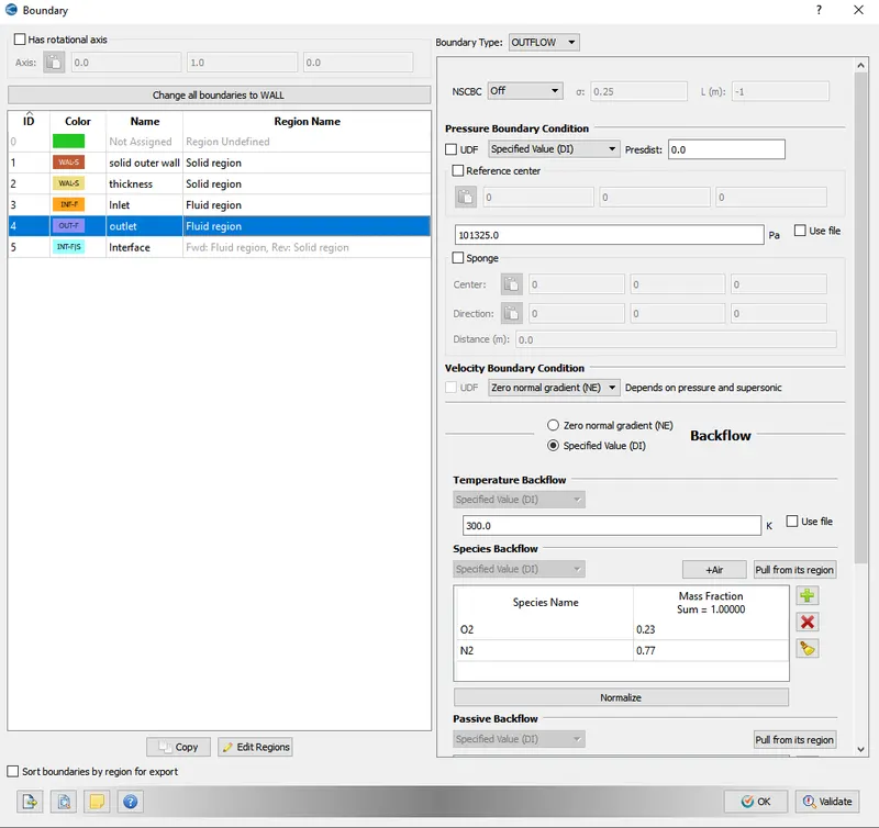
 For boundary type outflow: select the region as the fluid region. Pressure boundary is assigned 101325Pa and the velocity boundary condition as a zero normal gradient. 300K temperature as a backflow boundary condition. For species backflow, air is chosen.

Interface

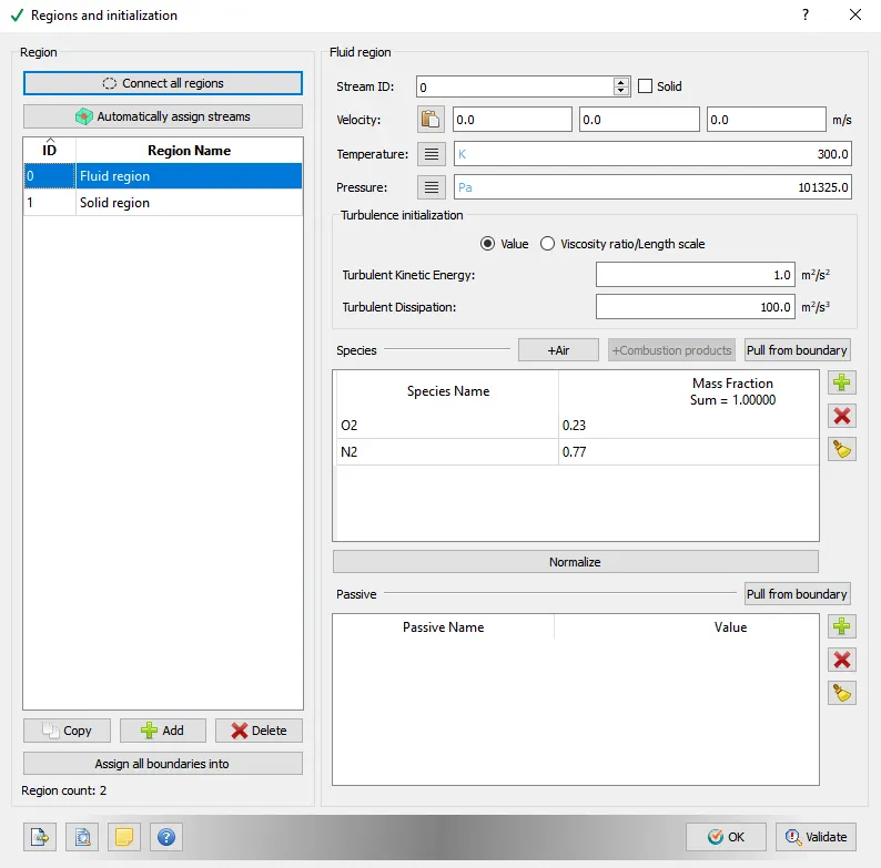
In Regions and Initializations, Region-0 and Region-1 are added as region.

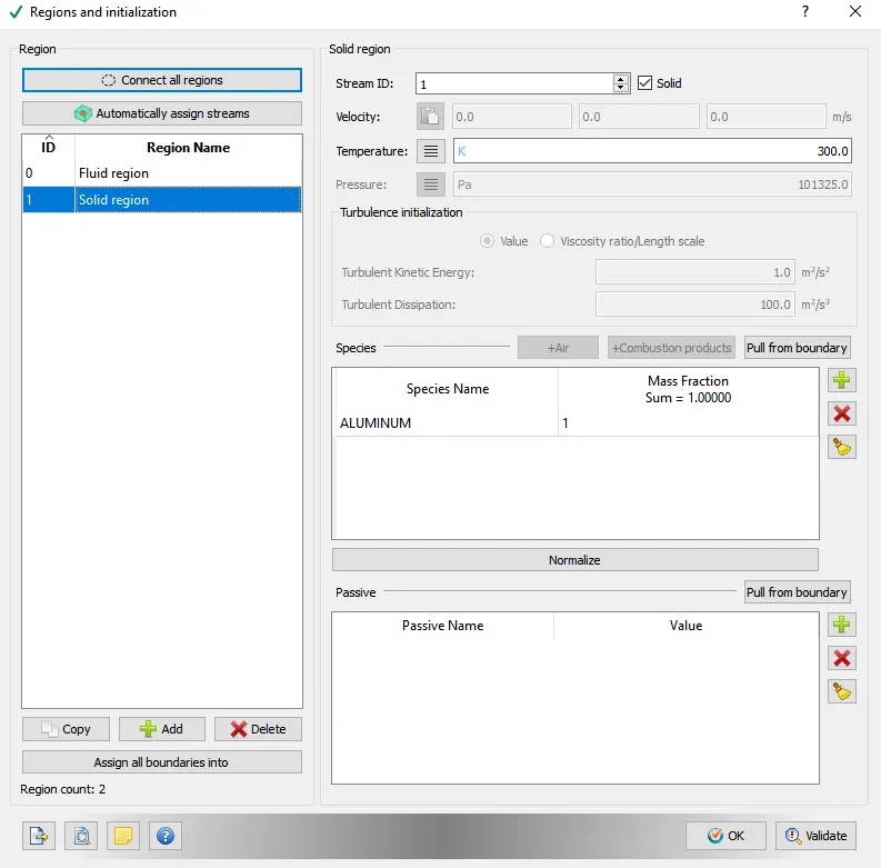
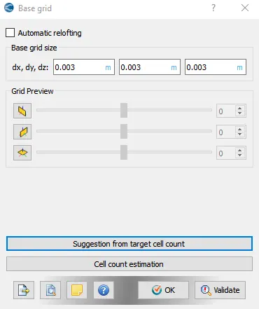
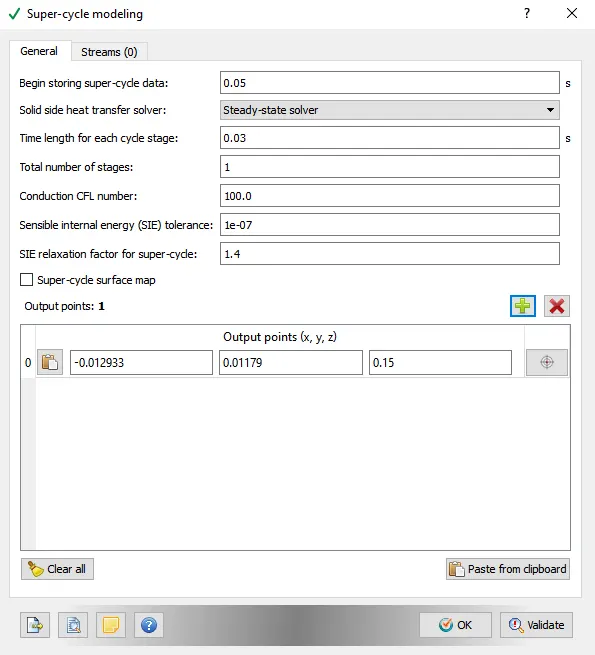
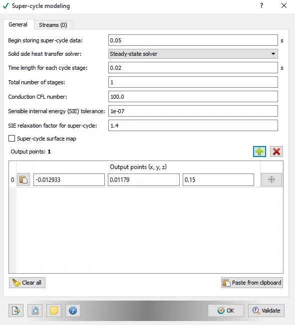
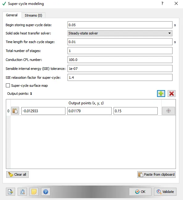
 The first option is to set the initial time at which the super-cycle begins storing data. This can be set from 0 to any value less than or equal to the total simulation time. The time length for each cycle determines the intervals at which the fluid domain is paused and the solid domain solved for. The CFL number, SIE tolerance and relaxation factors are solver parameters are assigned as default that are given for the purpose of accuracy and smooth running of simulation.An output point is assigned in the solid region to let the solver know at which the temperature data must be calculated. This point must be given in the solid domain as the solver runs for the solid domain and once this value converges, the fluid domain solver is continued. The simulations are run using using three base grid which is

• Case1:0.003( Case 1a,1b and 1c: Supercycle interval : 0.03,0.02 and 0.01)

Case 1a

Case 1b

Case 1c

• Case2: 0.002
• Case3: 0.0018

Now post variables are selected. In post variable selection Combustion/Turbulence is enabledwith default settings.

Solution and Post processing

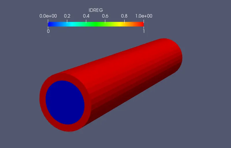
This is IDREG contour it displays the steam id selected during the solver settings with 1 being Solid region (red) and 0 being Fluid region (blue).

Grid Dependence test

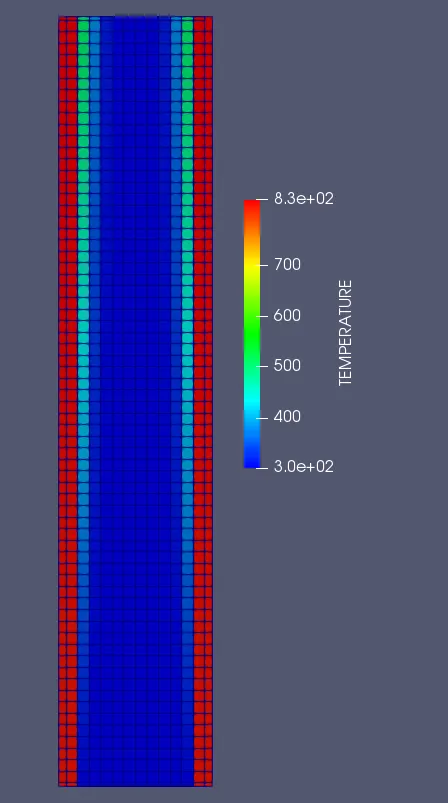
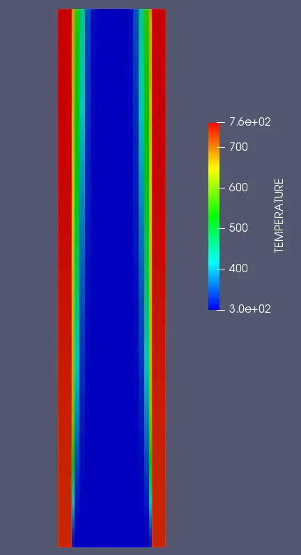
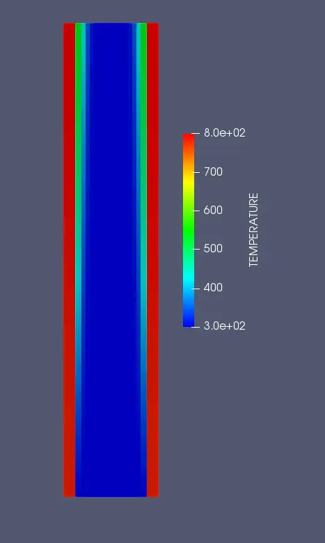
Temperature Contour : From the contour, if observed near the outlet side there are clear differences in all 3 grids. With more refinement the outlet temperature has converged to slightly different Values. Even the coloured profile observed in the base grid just below the solid region is less denser but as moved to grid 0.002 its more shaper and even more at the final grid 0.0018.

Case 1

Case 2

Case 3

Plot for Fluid & Solid Regions for all 3 grids.

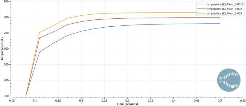
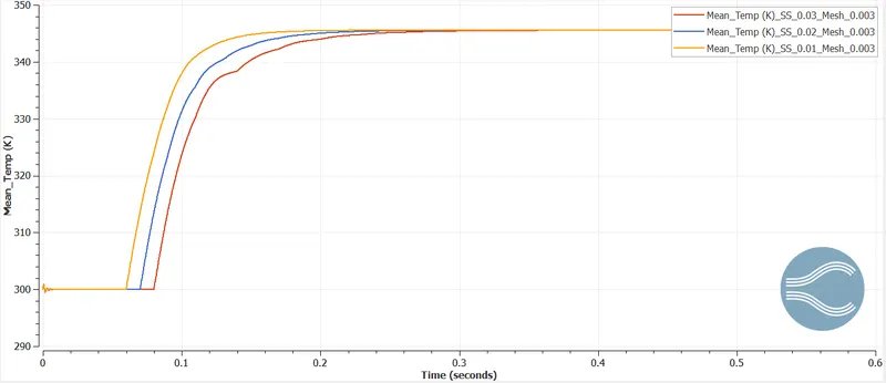
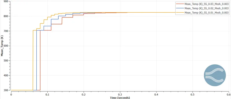
Mean temperature plots for all 3 grids for fluid and solid region separately are shown below, each converging to slightly different values. The effect of super cycling can be seen in the Solid region plot. The assigned location in the solid region where the value remains stable is being averaged then steady state solver runs and averages it to a updated converged value.. The grid is temperature dependent and further refinement would most likely give a highly refined output.

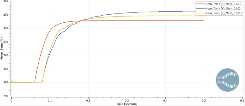
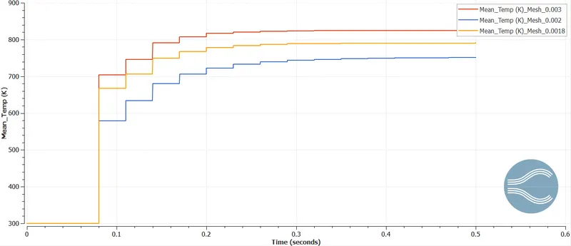
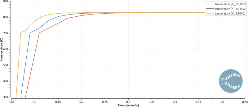
Effect of addition of a particular Super cycle stage interval of 0.03 for the 3 grid sizes on the monitor point: The Supercyle affects the time to solve the equations and reach convergence. The ss effect for grid size 0.002 seems to have converged rapidly to a the least temperature followed by increased temperature for 0.002 and 0.0018. By oberving the above plots we can easily say that at the finer mesh we got the more accurate values of temperature. But at the finer mesh computational effort has been increased.

 

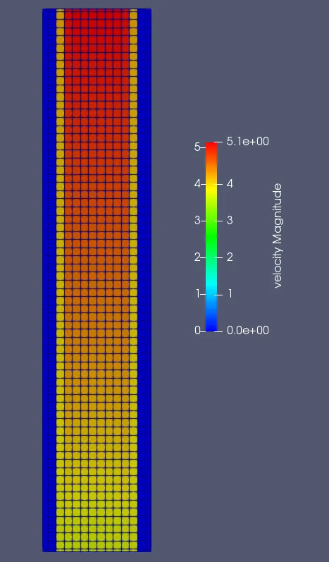
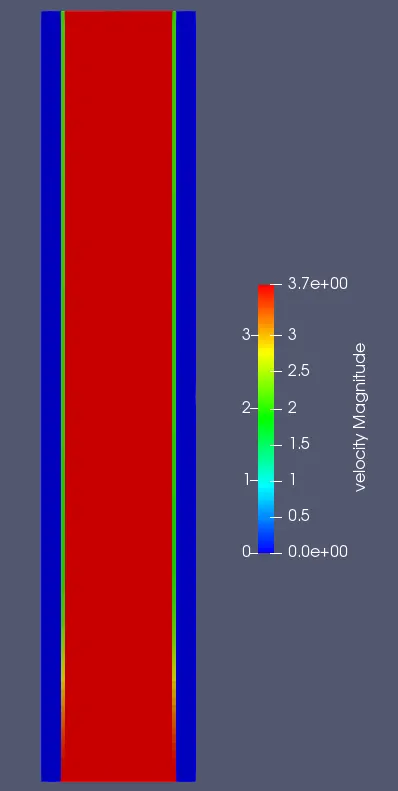
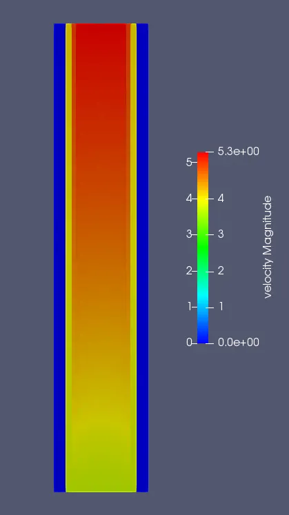
Velocity contours for all the 3 grid sizes:

Case 1

Case 2

Case 3

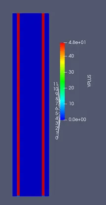
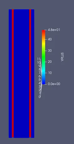
Y+ contour for all the 3 grid sizes.

Case 1: Y+ value=48

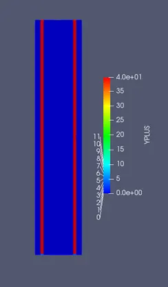
Case 2: Y+ value=40

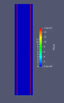
Case 3: Y+ value =16

Effect of variation of Supercycle stage interval for the base mesh on the mean fluid temperature and solid temperature and the sole effect of supercycle on the monitor point: The plot as can be seen the cycle stage starts at the second set for super cycling and converges to a same temperature at the end of convergence. This means that the solution for same mesh is supercycle independent for these particular values. However the time taken to solve these 3 varies and once we know this then we can use super cycling value interval to reach steady convergence faster in future. In the above plots, we can easily observe that setting the lower value of supercycle stage interval converges to the exact values of temperatures. Basically we increase the value of supercycle stage interval from 0.01 to 0.03. we got the more exact values at 0.03 supercycle stage interval.

Fluid side Mean Temperature

Solid side Mean Temperature

Supercycle stage interval effect on the monitor point:

Supercycle stage interval effect on Y+

Case 1a, Case 1b, Case 1c : same value for all the 3 cases(no effect) i.e 48

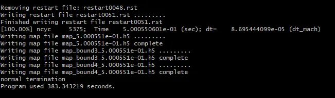
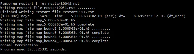
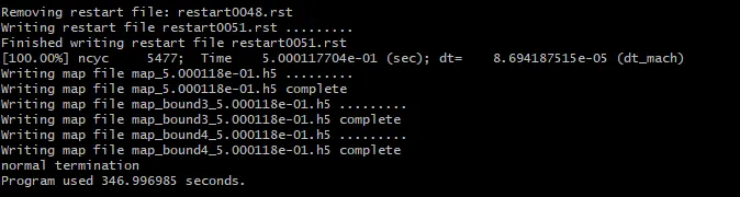
Supercycling simulation time:

Case 1a

Case 1b

Case 1c

Animation:

Case 1

Case 2

Case 3

Results discussion of the effect of supercycle stage:
We set the supercycle stage interval, i.e time length for each cycle stage from supercycle modelling is used 0.01, 0.02 and 0.03. And for smallar value of supercycle stage interval the convergence is achieved faster.  Super-cycling is done as the heat flow in the solids when depicted by a transient solver, is time consuming. Hence it is better to apply steady-state analysis for the heat transfer through the solid while studying the behaviour of fluid flow through the pipe by runniong transient solver which is paused andf the steady state solver for the solid is ran and made to converge followed by the running of transient solver fluid region.

Temperature profile in the solid region
The steady state solver is employed in the solid region resulting in the sudden increase in temperature at various time intervals. This does not represent the actual temperature flow in the solid and only the steady-state
temperature. It is to be noted that the increase in the temperature in the solid regions is due to the heat flux added to the solid outer wall. For the Temperature profile in the fluid region the transient solver is used to simulate the flow in the fluid region which is the cause for actual increase in the temperature in fluid region. The increase in temperature is due to the transfer of heat from the solid to the fluid.