CONJUGATE HEAT TRANSFER SIMULATION OF A SOLID PIPE HEATED BY AN EXTERNAL FLUX USING CONVERGE CFD
Aim: Simulate conjugate heat transfer for air flowing through an aluminium pipe.
1. Run a grid dependence test for the given problem
2. Analyse the effect of supercycle stage interval on the simulation time
Introduction and Theory:
Conjugate Heat Transfer is a process which involves temperature variations in solids and fluids due to the thermal interaction between them. In solids conduction dominates, whereas in fluids convection ususally dominates. Efficiently combining heat transfer in fluids and solids is the key to designing effective coolers, heaters, or heat exchangers. Forced convection is the most common way to achieve high heat transfer rate. CHT can be performed to improve cooling performance of the water jacket and increase engine life. Conjugate Heat Transfer analysis provides the temperature distribution in solid and coolant of the engine and the velocity distribution and mechanism of heat transfer of coolant. Results of CHT analysis become input to structural simulations as thermal loads.
Converge solves the fluid heat transfer using the Navier-stokes energy equation and solid heat transfer using the solid heat equation.
Geometry :
The geometry for the simulation is created in Converge CFD software and the boundaries are flagged accordingly such as the inlet, outlet, solid outer wall, interface, solid side.
Note: The interface boundary is the boundary which is located in between the solid pipe and fluid flow area. Hence named as the interface.
Calculation of Grid size
Reynolds Number Re = 7000
Density of air (@ 300K and 1atm) = `rho = 1.1766 {kg}/m^3`
Dynamic Viscosity (@ 300K and 1atm) `mu = 0.00001846 {kg}/{ms}`
Kinematic Viscosity = `mu/rho = 1.56893E-05 {m^2}/s`
Pipe inner diameter = d = 0.03 m
Average flow velocity `=(Re*mu)/(rho*D) = 3.66 m/s`
Skin friction drag coefficient = `C_f =0.0576*Re^(-1/5)= 0.00980399`
Wall Shear Stress `tau_w = Cf*{rho*v^2}/2 = 0.077296708 N/m^2`
Frictional Velocity = `u_t = sqrt(tau_w/rho) = 0.256310311 m/s`
Assuming the desired Y+ = 32
Then first cell centre to boundary distance = `Y_{+}*nu/{u_t} = 0.001958785 m`
Cell Size = 2*0.001958*1000 = 3.92 mm ~= 4mm
Case Setup:
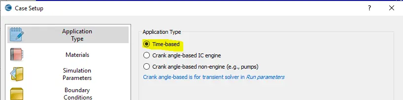
Application type is selected as time based
Materials: Keep Gas simulation and Solid simulation both enabled.
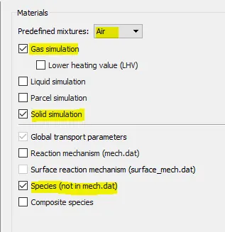
Gas Simulation: Keep equation of state as Redlich-Kwong and keep all other parameters as default.
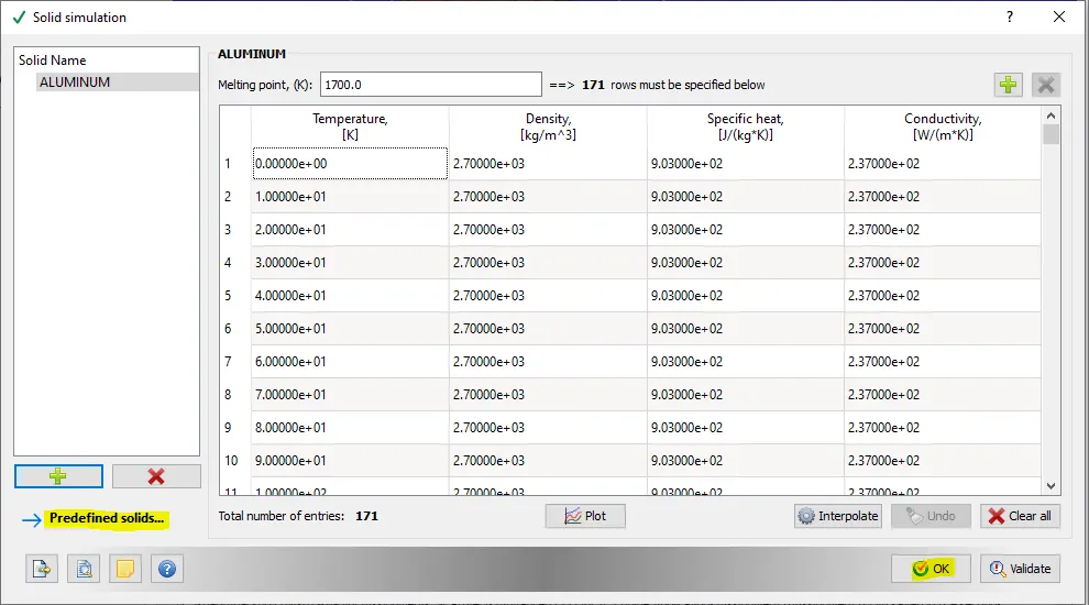
Solid Simulation: From predefined materials select aluminium.
Global Transport Properties: Keep all the values default.
Species: Under Gas tab select O2 and N2 as gas species, Under Solid tab select aluminium as species.
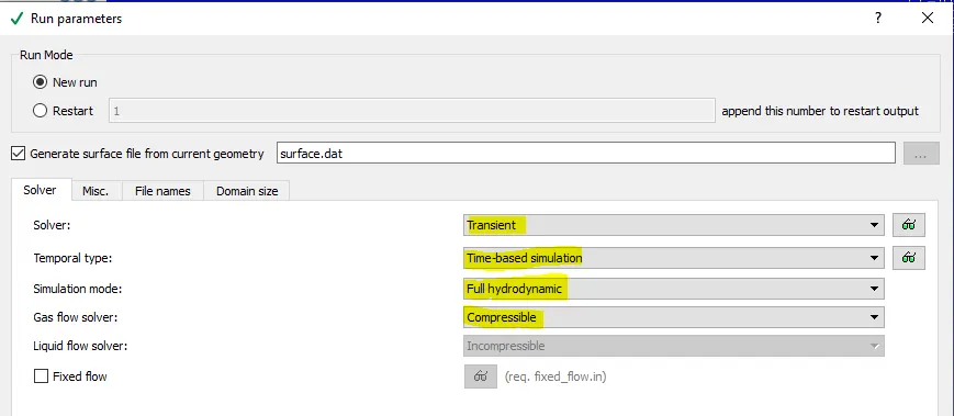
Run Parameters: Under run parameters, keep the solver type as Transient, Time-based simulation, Full Hydrodynamic, and compressible.
Disable shared memory flag under misc. tab.
Simulation Time Parameters
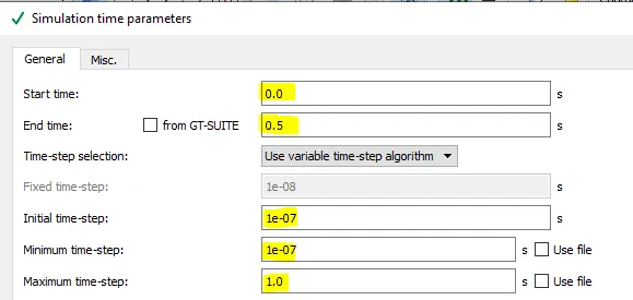
Start time as 0, end time as 0.5 s, Initial and Minimum time step as 1e-7 and max time step as 1 second.
Solver Settings
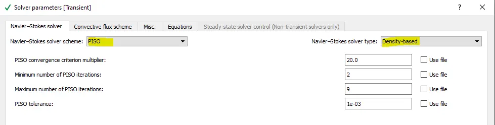
Keep all the settings default.
Boundary Conditions
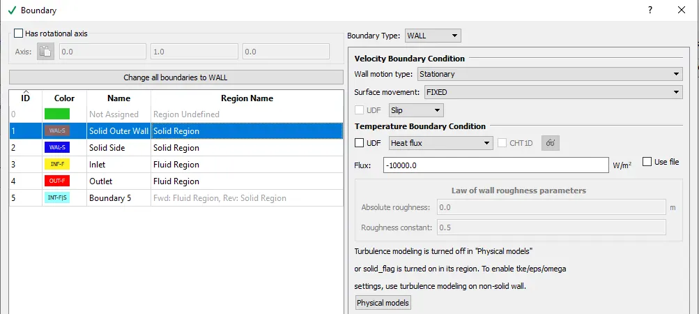
Solid Outer Wall
Select the region as solid region. Boundary Type as Wall, Velocity boundary condition as slip, temperature boundary condition as Heat Flux of 10000 W/m^2
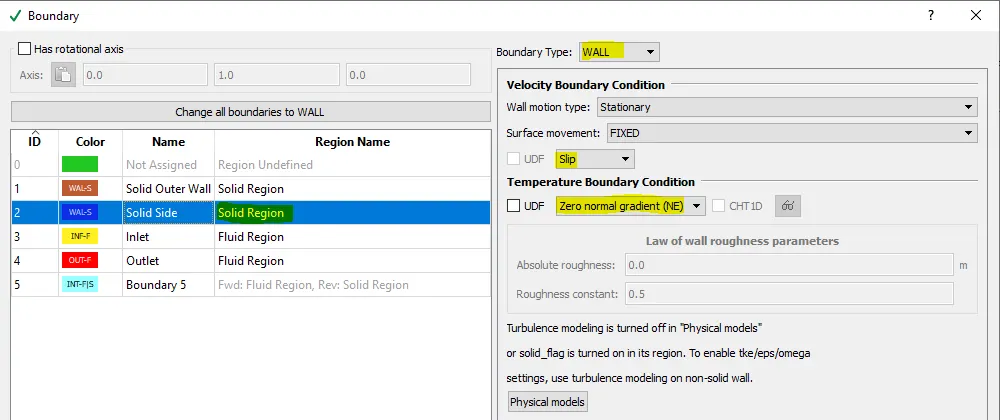
Solid Side walls
Select the region as solid region. Boundary Type as Wall, Velocity boundary condition as slip, temperature boundary condition as Zero Normal Gradient.
Inlet
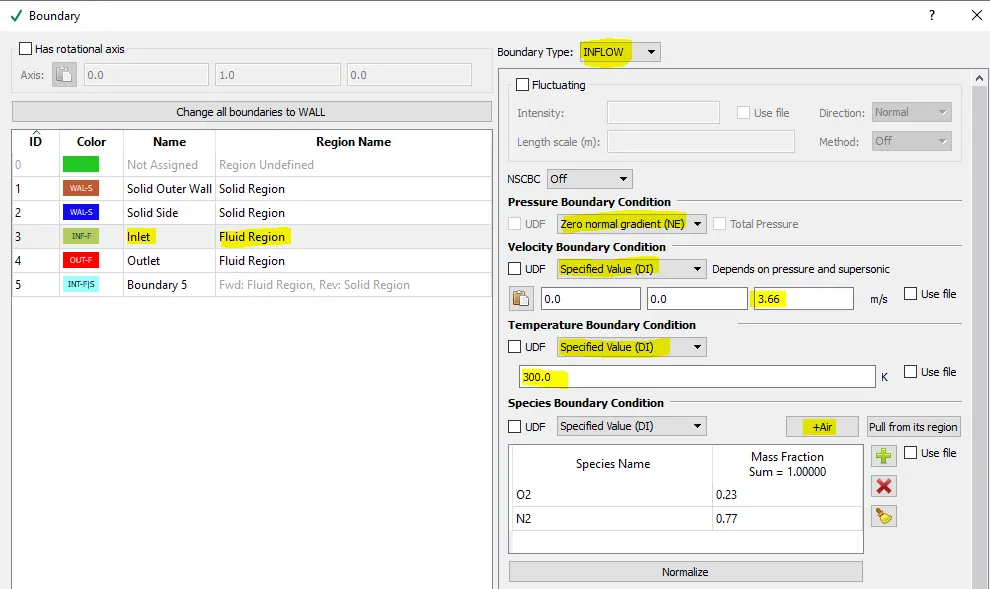
Select the region as fluid region. Boundary Type as Inflow, Pressure boundary condition as Zero Normal Gradient, Velocity boundary condition as specified value of 3.66 m/s in positive Z direction, temperature boundary condition as specified value of 300 K and for Species boundary condition select Air.
Outlet
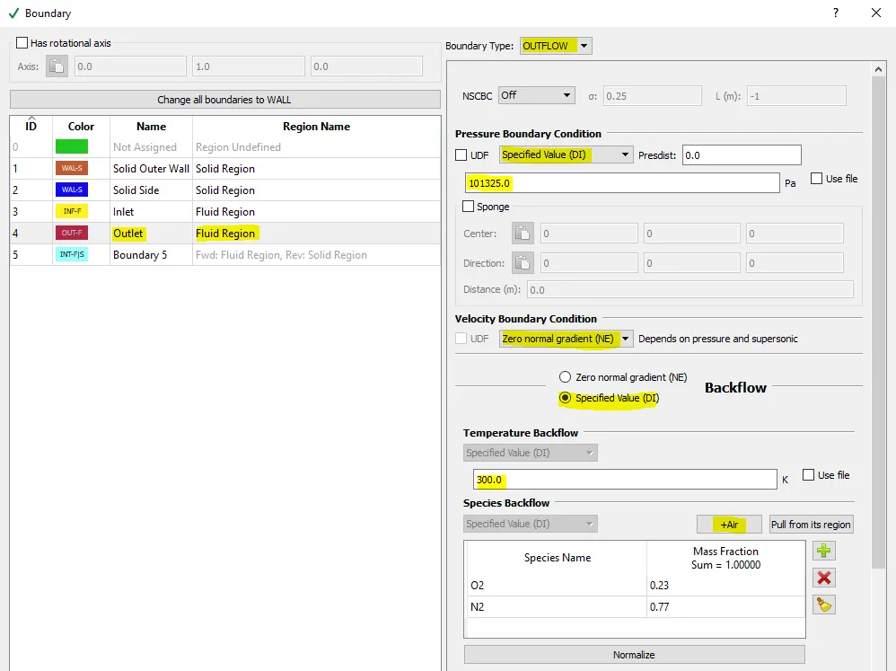
Select the region as fluid region. Boundary Type as Outflow, Pressure boundary condition as Specified Value of 101325 Pa, Velocity boundary condition as Zero Normal Gradient, temperature backflow boundary condition as specified value of 300 K and for Species Backflow boundary condition select Air.
Interface Boundary
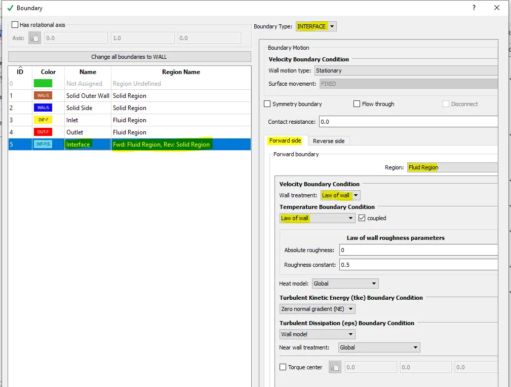
Select the boundary type as Interface.
Forward Side
For Forward Side select the region as Fluid Region, Velocity and Temperature boundary condition as Law of Wall.
Backward Side
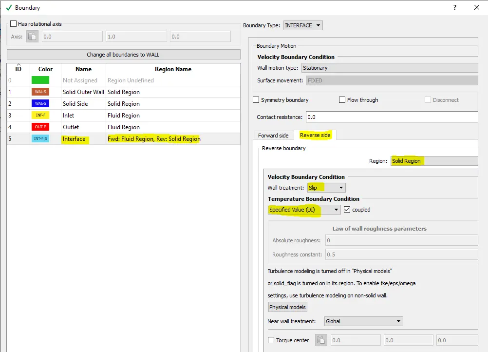
For backward Side select the region as Solid Region, Velocity Boundary condition as Slip and Temperature boundary condition as Specified Value.
Regions and Initialization
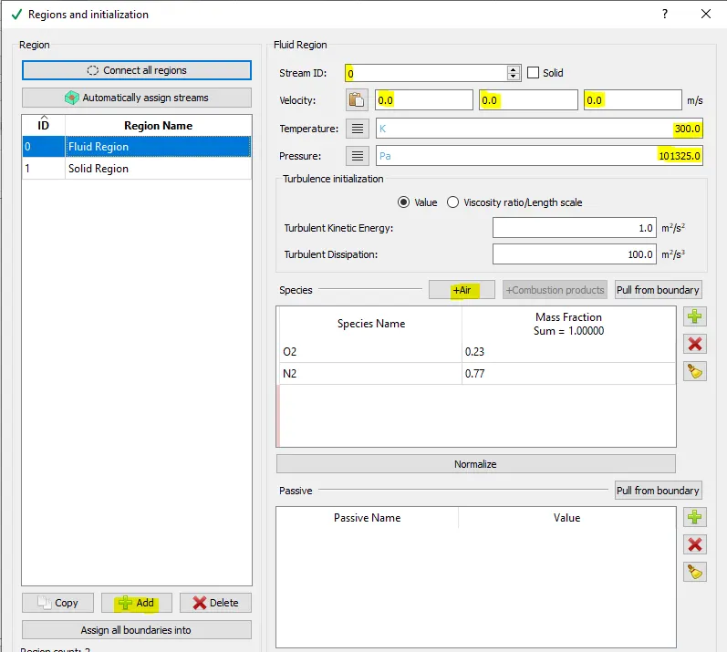
Add 2 Regions, name them solid region and fluid region.
For the Fluid Region set the Stream ID as 0 velocity initial conditions (0, 0, 0) m/s, Temperature initial conditions as 300 K, Pressure Initial condition as 101325 Pa.
Select Species as Air
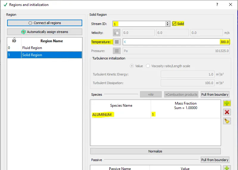
For the Solid Region, select the Stream ID as 1, Keep Solid check box enabled.
Set the temperature boundary condition as 300K. Species boundary condition as Aluminium with a mass fraction of 1.00.
Physical Modelling
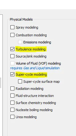
Just keep Turbulence modelling and Super-Cycling modelling enebled.
Turbulence Modelling: Keep the turbulence model as `"RNG "k-epsilon` model with all default values.
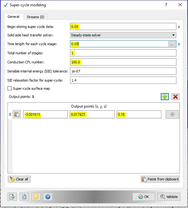
Super Cycle Modelling
Set the following values for super cycling modelling. Select a point for measuring the temperature convergence near but before the outlet inside the mid of solid region thickness.
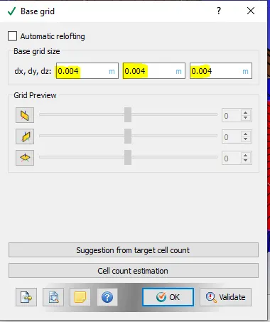
Grid Size
Set the calculated grid size of 4 mm.
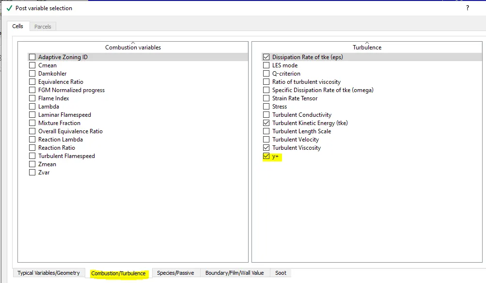
Post Variable selection
Include the variable Y+ for the simulation from Combution/Turbulence tab.
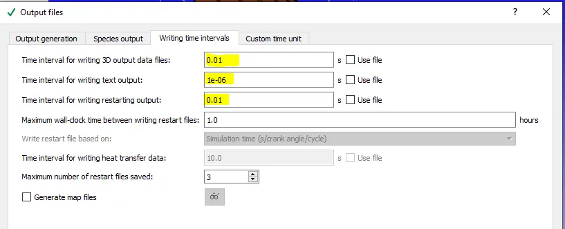
Output Files
Set the following values for the frequency of writing the output data (3D output, text output, and restart files.)
Results of Simulation (Grid Dependence Test):
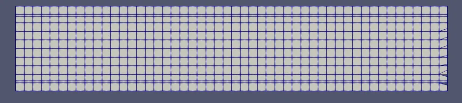
Case 1: Mesh Size of 4 mm
Mesh
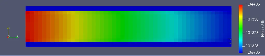
Pressure Profile
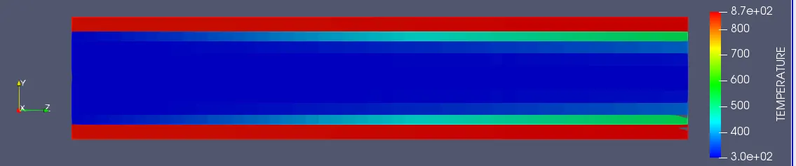
Temperature Profile
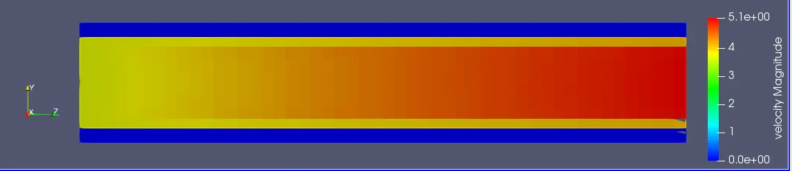
Velocity Profile
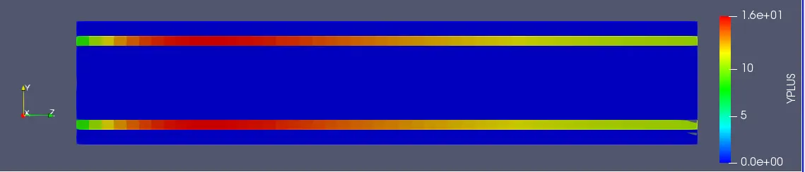
Y+ Profile
Mean Temperature vs Time plot
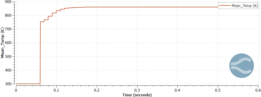
Final Mean Converged Temperature = 860.59 K
Case 2 Mesh Size = 3mm
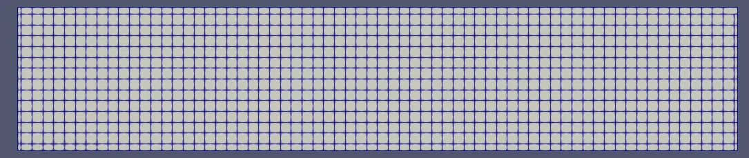
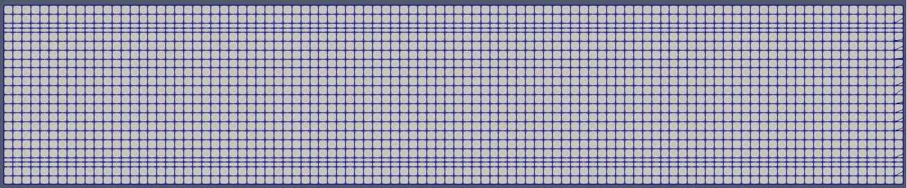
Mesh
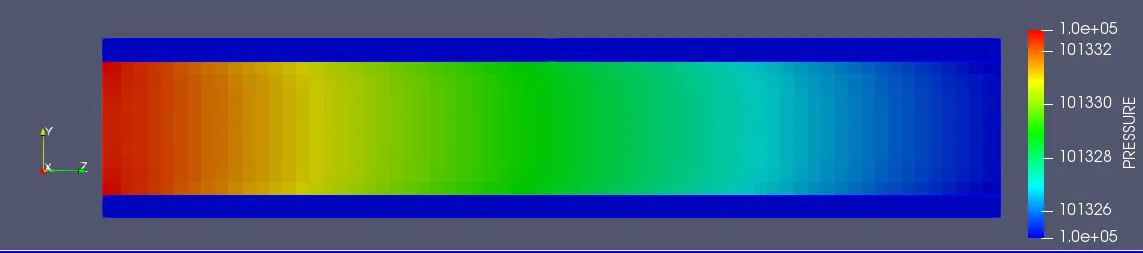
Pressure Profile
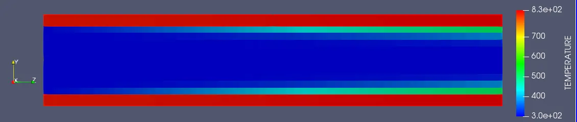
Temperature Profile
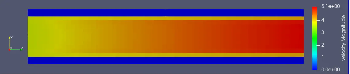
Velocity Profile
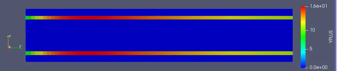
Y+ Profile
Mean Temperature vs Time plot
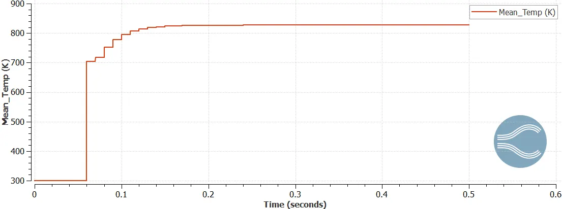
Final Mean Converged Temperature = 827.08 K
Case 3: Mesh Size = 2 mm
Mesh
Pressure Profile

Temperature Profile

Velocity Profile

Y+ Profile

Mean Temperature vs Time Plot
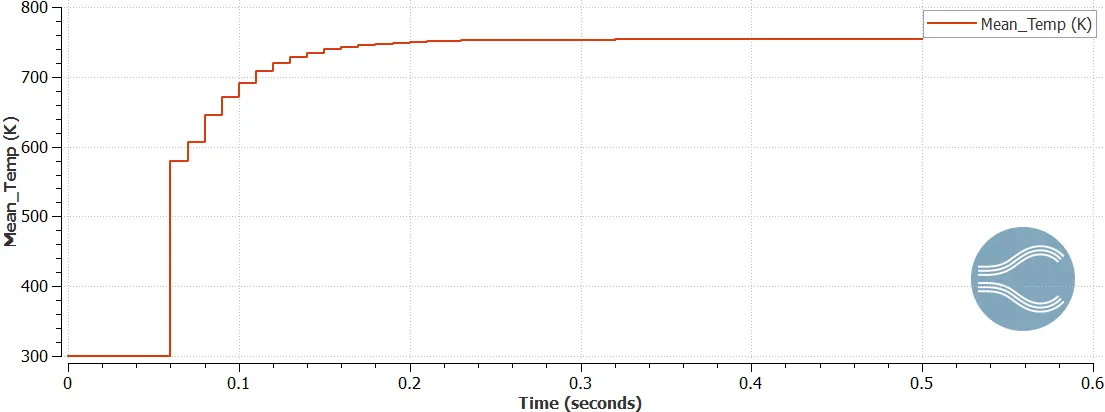
Final Mean Converged Temperature = 753.6 K
Results of Simulation (Effect of Supercycle Stage Interval on Simulation time)
Case 1: SuperCycle Stage Interval = 0.01
Mesh
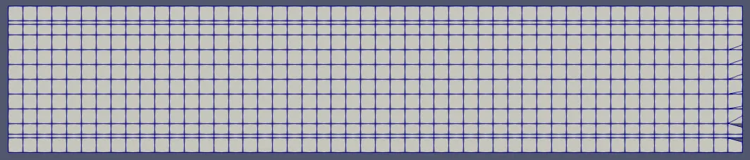
Pressure Contour

Temperature Contour

Velocity Contour

Mean Temperature vs Time Plot
Final Mean Converged Temperature = 860.62, Convergence achieved after about 0.18 seconds
Case 2: SuperCycle Stage Interval = 0.02
Mesh
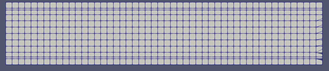
Pressure Contour

Temperature Contour

Velocity Contour

Mean Temperature vs Time Plot
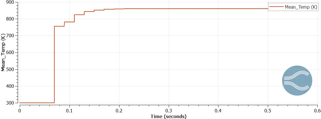
Final Mean Converged Temperature = 860.599 K, Convergence achieved after about 0.23 seconds
Case 3: SuperCycle Stage Interval = 0.03
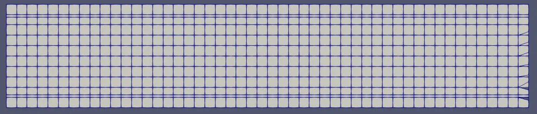
Mesh
Pressure Contour

Temperature Contour

Velocity Contour

Mean Temperature vs Time Plot
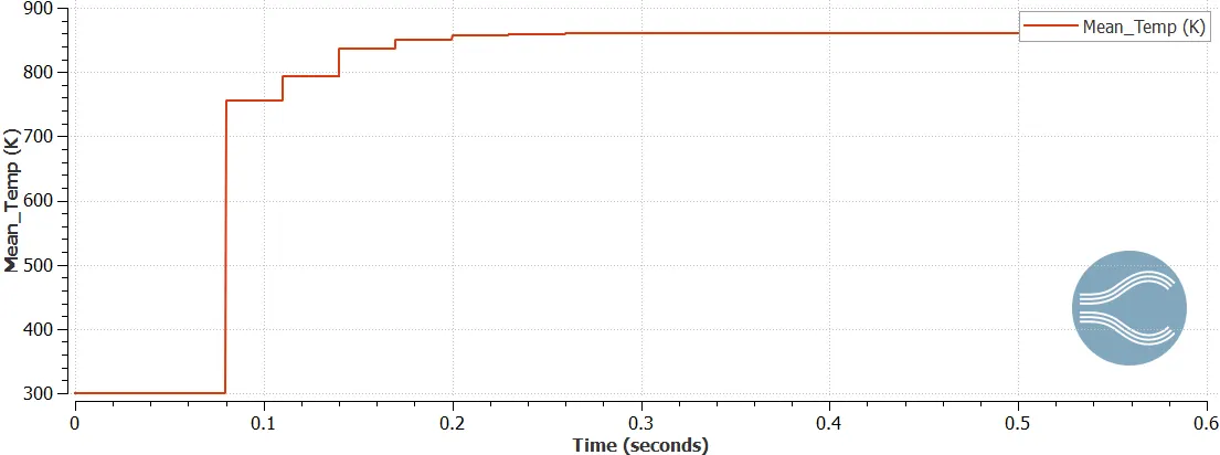
Final Mean Converged Temperature = 860.57 K, Convergence achieved after about 0.3 seconds
Pressure Contour
Temperature Contour
Velocity Contour
Observation from the above results:
Grid Dependency Test
1. Y+ decreases as we decrease the mesh size, Y+ range for 2mm mesh varies from 0 to 7.3 whereas Y+ for 4mm mesh varies from 0 to 16
2. As we decrease the mesh size the flow in viscous layer close to the wall are more accurately captured.
3. For a finer mesh size the converged value of mean temperature is the lowest (753.6 K) and it is the accurate value compared to 3mm and 4mm mesh size results.
Effect of SuperCycle Stage Interval on Simulation Time
For smaller value of supercycle stage interval the convergance is achieved faster and simulation time is also less.
For Case 1, SuperCycle stage interval of 0.01 convergance time is about 0.18 seconds and simulation time is 1688 seconds
For Case 2, SuperCycle stage interval of 0.02 convergance time is about 0.23 seconds and simulation time is 1932 seconds
For Case 3, SuperCycle stage interval of 0.03 convergance time is about 0.3 seconds and simulation time is 2166 seconds
Conclusion:
A simulation of conjugate heat transfer in air flowing through a pipe heated with constant heat flux was setup and run in Converge CFD. Various contour plots of Pressure, Velocity, Temperature and Y+ were studied.
A grid dependency test was done with 3 different mesh sizes and the effect of SuperCycle stage interval on the simulation time was studied.