Week 6: Conjugate Heat Transfer Simulation
Objective:
- Setup a flow simulation through a pipe
- Perform grid dependence test
- Compare the effect of the supercycle stage interval
Geometry
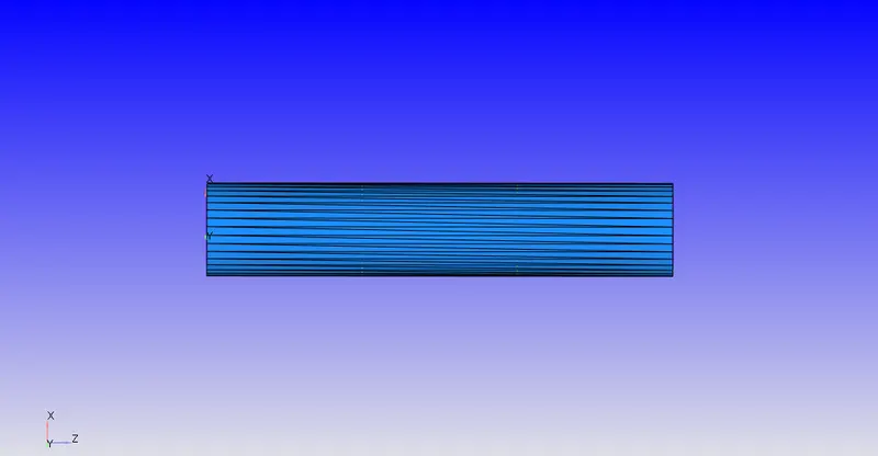
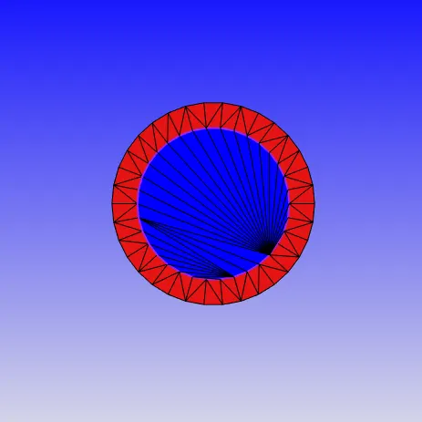
The geometry is created using the create cylinder shape option in converge studion.
Inner radius=0.015m
Outer radius=0.02m
Case setup
Application type: Time based
Species:
Gas: N2, O2
Solid: Aluminium
Run parameters
Solver: Transient
Simulation mode: Full hydrodynamic
Gas flow solver: compressible
Simulation time parameters
Start time= 0s
End time=0.5 s
Initial time step= 1e-7
Minimum time step= 1e-7
Maximum time step=1
Solver parameters
Navier stokes solver scheme: PISO
Navier stokes solver type: Density-based
Boundary conditions
Solid outer wall: Wall BC
Heat flux=-10000 W/m2
Solid wall thickness: Wall BC
Temperature Bc= Zero normal gradient
Inlet: Inflow BC
Inlet velocity is calculated from the given Reynolds number.
`Re= (rho*V*D)/mu`
Given, Re=7000,
For `rho and mu` we can take the values for air at room temperature.[Flowing fluid is given as air]
So the inlet velocity,
Velocity= 2.7m/s
Outlet: Outflow BC
Temperature=300 K
Pressure=101325.0 Pa
Interface: Interface BC
Regions and Initialization
| Region | Species | Mass Fraction | Pressure(Pa) | Temperature(K) |
| Solid | Aluminum | 1 | -- | 300 |
| Fluid region |
O2 N2 |
0.23 0.77 |
101325 |
300 |
Physical models
Turbulence model= RNG k epsilon
Since it is a Conguhate heat transfer simulation supercycle modeling is used. In order to understand the effect of supercycle stage intervals on the solution, The simulation is run for three different supercycle stage intervals 0.03,0.02,0.01 respectively.
Grid
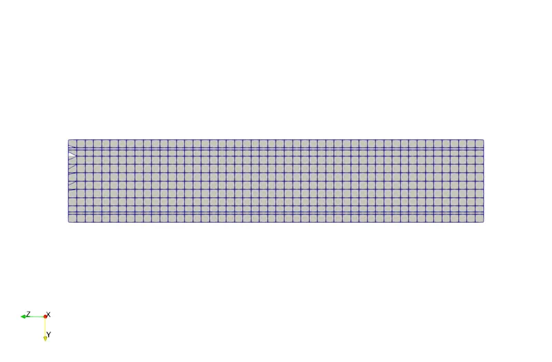
Base grid size=0.04 m
Results
Grid dependence
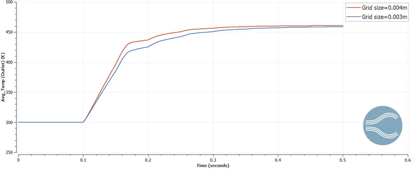
For testing the grid dependence. The simulation is run for two different mesh sizes. Base grid size=0.004m and 0.003m the plot of average outlet temperature for the two cases shown below. The final value of the average temperature converges to almost 459K.
Velocity contour
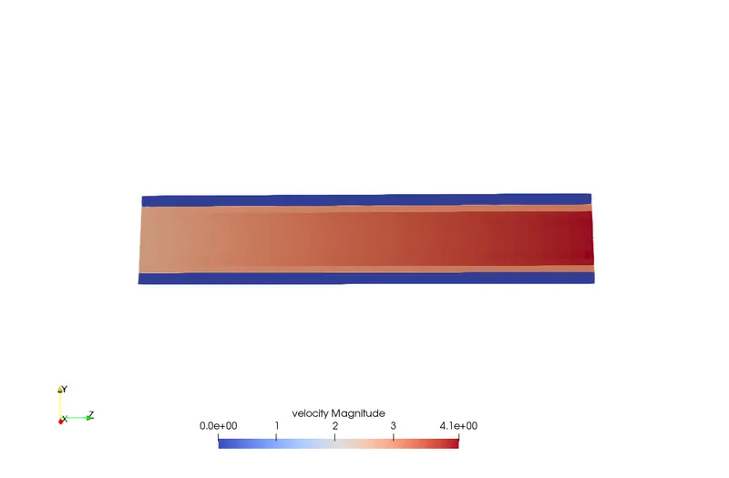
From the above plot, we can see the boundary layer formation near the wall. Since embedding is not added the boundary layer is to captured well.
Pressure contour
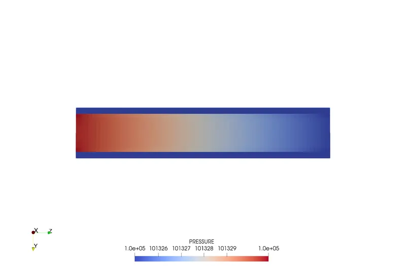
Pressure contour plotted on cut plane x is shown below,
Temperature contour
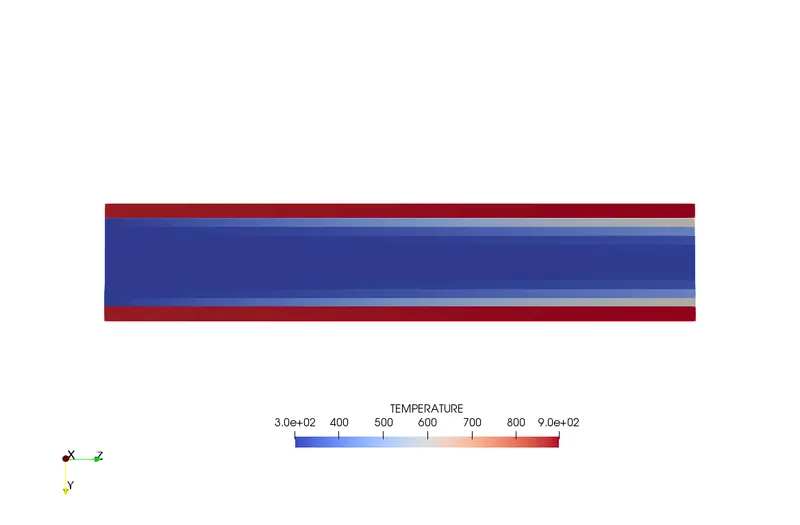
From the above plot, we can see that near the inlet temperature is low and near the outlet temperature increases due to the heating from the solid pipe.
Effect of supercycle stage interval
The simulation is run for three different stage interval values and the average outlet temperature is plotted.
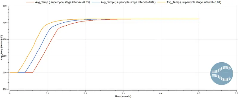
From the plot, The final temperature for the three cases is the same. The final temperature is independent of the supercyclic stage interval. But the final temperature converges fast when the stage interval is low.
Y+ plot
Temperature animation
Velocity animation