Week 6: Conjugate Heat Transfer Simulation
AIM: TO SIMULATE CONJUGATE HEAT TRANSFER IN A PIPE AND STUDY THE EFFECTS OF SUPERCYCLING USING CONVERGE.
What is conjugate heat transfer?
Conjugate heat transfer corresponds with the combination of heat transfer in solids and heat transfer in fluids. In solids, conduction often dominates whereas in fluids, convection usually dominates. Conjugate heat transfer is observed in many situations. For example, heat sinks are optimized to combine heat transfer by conduction in the heat sink with the convection in the surrounding fluid.
GEOMETRY:
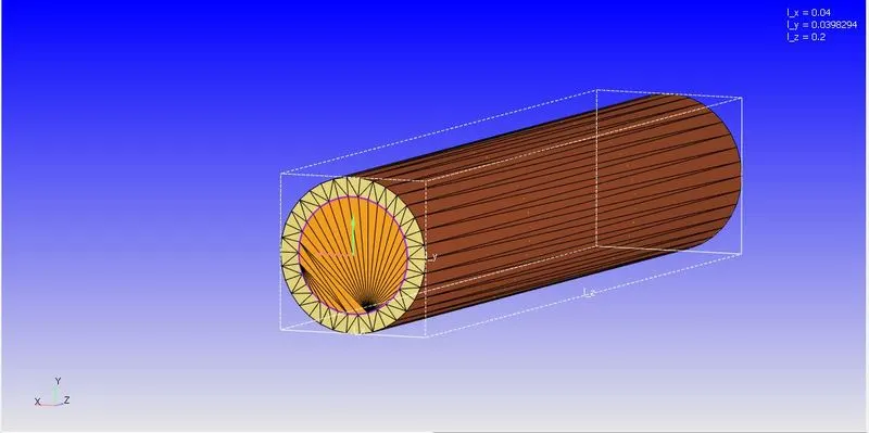
This geometry was created on Converge 3.0 using the Create --> Shape--> Cylinder. The dimensions were mentioned as required thus resulting in the formation of the geometry.
Dimensions:
Outer Cylinder:
length: 0.2m
Diameter:0.04m
Inner Cylinder
length: 0.2m
Diameter:0.03m
Case Setup:
Procedure to setup the case:
- Select time based in the application.
- Here, we opt for solid and gas simulation as we are simulating a conjugate heat transfer model which involves heat transfer between two domains.
- Also we setup the specied module for both the gas as (`N_2` and `O_2`) and Solid as Aluminum.
- In the simulation parameters, we select the transient solver, timme based solver and make sure that the mode of simulation is full hydrodynamic. (Usually, simulations are run in non-hydrodynamic mode to ensure that the grid formed on the case is as expected. Due to the simplicity in the geometry, we directly use the full hydrodynamic mode.)
- We setup the boundaries as required also we assign the region to each of the boundary.
- In this case, we assign 2 regions. This is because we are dealing with two interfaces (ie. solid and liquid).
- Also different stream ID's were assigned to differentiate the above. In the solid region the solid check box was checked to ensure that the data of the solid chosen is imported.
- Here we employ the turbulence modeling where we use the RANS method and we use the RNG k ε.
- The most important aspect in this model is to make sure that the model is dimentioned in meters. Also the base grid dimensions are to be mentioned in meters.
- We employ Super cycling in order to ensure that the simulation takes place sooner.
- The post processing is done on the results once the simulation is complete.
Few particulars:
Outer wall : 10000 `W/m^2` (constant heat flux)
Inlet velocity: 2.78 m/s
outlet pressure:101325.0 Pa
Species Boundary conditions:
Gas:
O2= 23%
N2">N2=77%
Solid:
Aluminum:
mass fraction =1
Simulation parameters
Start Time: 0 sec
End Time (sec)= 0.5 sec
minimum time steps=1e-7s
maximum time step=1s
Calculation of Inlet velocity:
`Re = (rho.V.D)/mu`
`rho =" density of air at 300k"=1.161 (kg)/m^3`
`Re=" Reynolds number"=7000`
`V="velocity"`
D= diameter = 0.04m
`mu="dynamic viscosity"=1.846 * 10^-5 (kg)/m s`
The velocity was found to be 2.78m/s
To study the variations in super cycling and grid dependancy, the following are the cases:
SUPER CYCLE STAGE
case 1: 0.05s
case 2: 0.01s
case 3: 0.02s
case 4: 0.03s
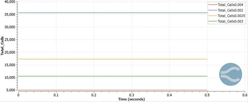
GRID SIZES:
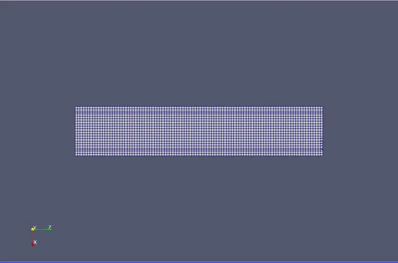
case 1: 0.002m
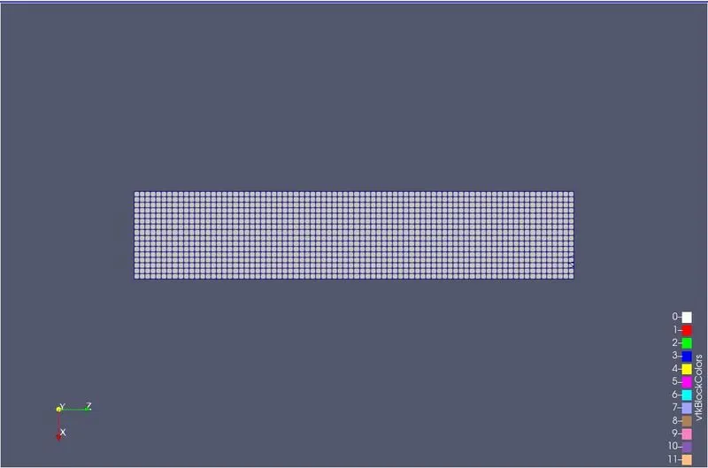
case 2: 0.0025m
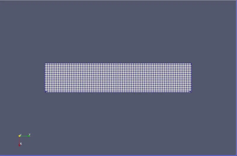
case 3: 0.003m
case 4: 0.004m
Grid Dependancy Test:
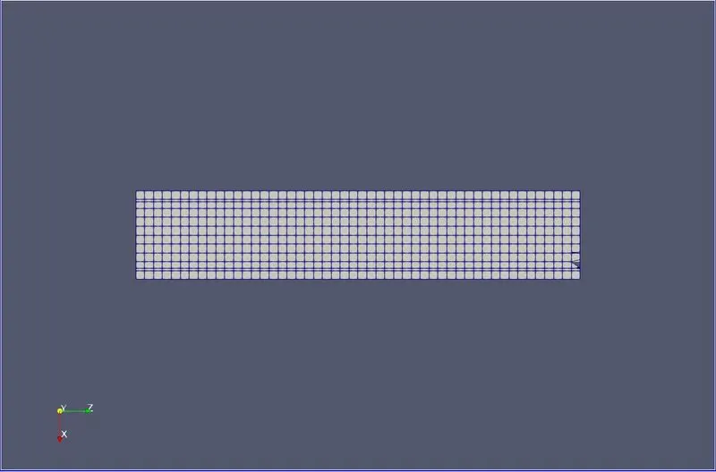
Meshes:
case 1:
case 2:
case 3:
case 4:
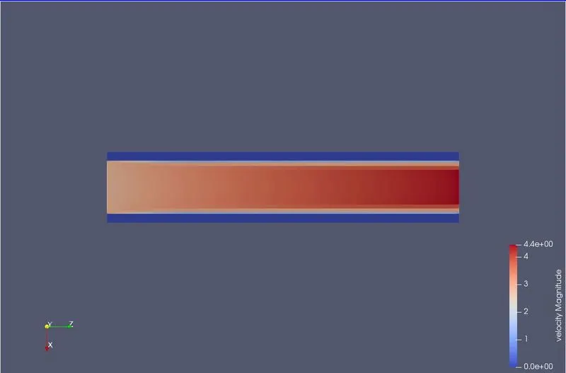
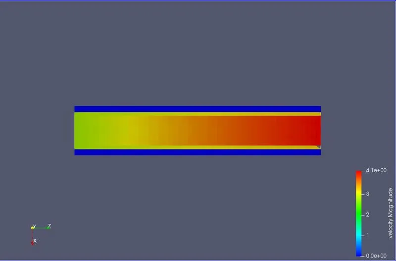
Velocity Profiles:
case 1:
case 2:
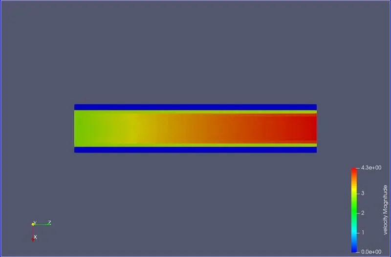
case 3:
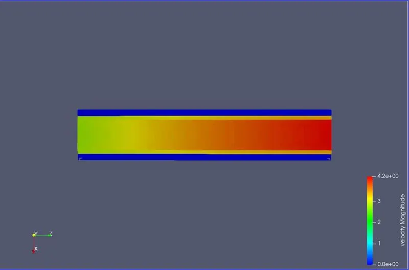
case 4:
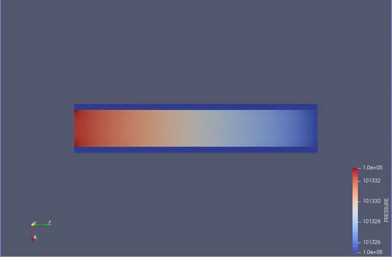
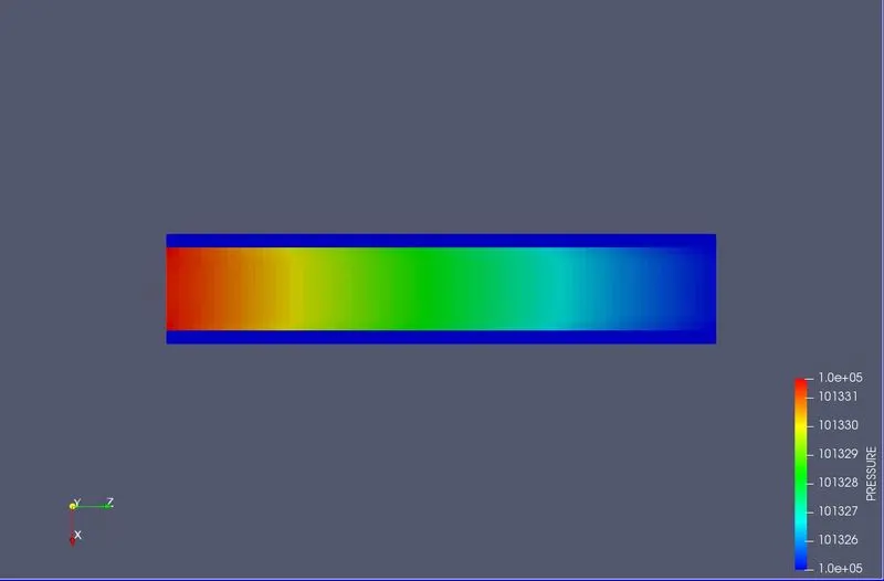
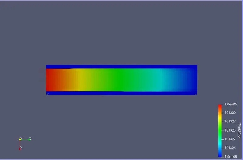
Pressure Profiles:
case 1:
case2:
case 3:
case 4:
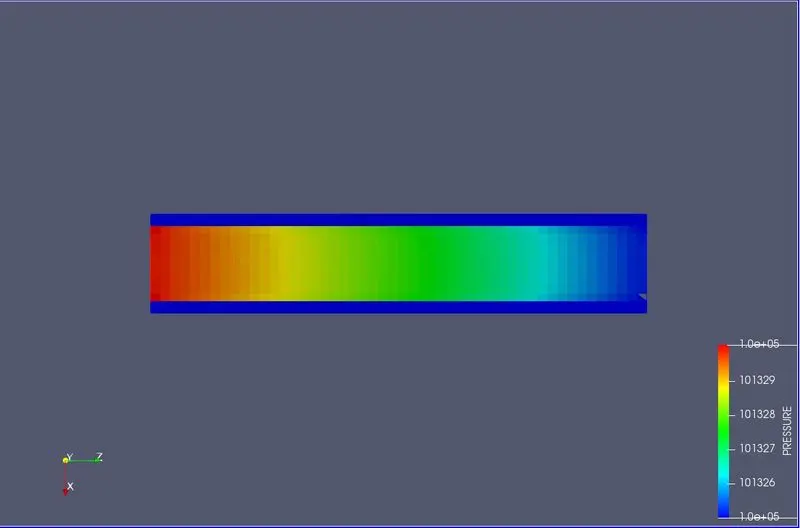
Temperature profile:
case 1:
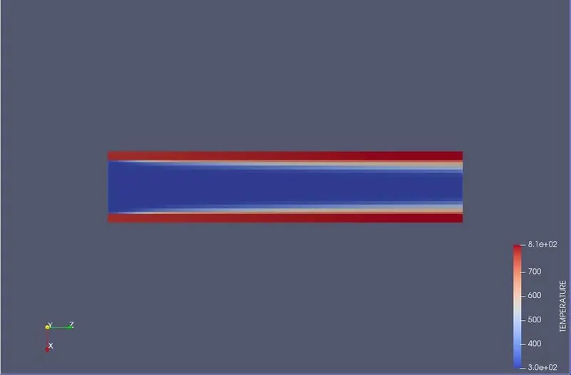
Case 2:
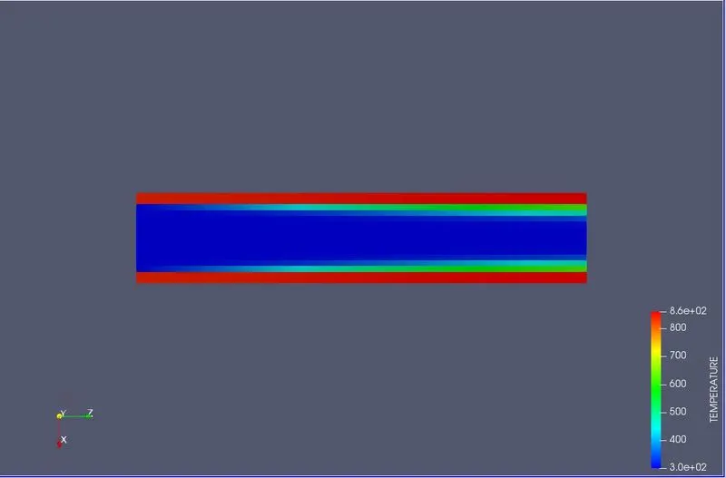
case 3:
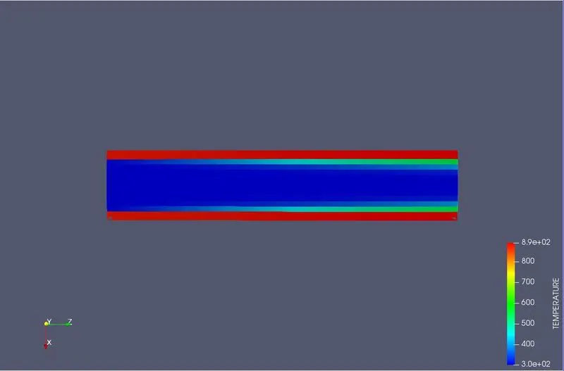
case 4:
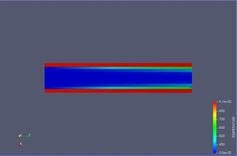
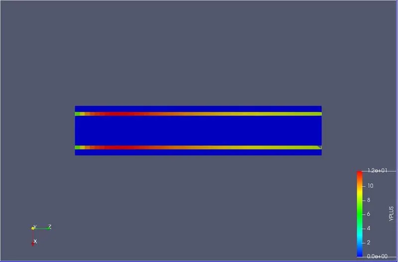
Y Plus profiles:
case 1:
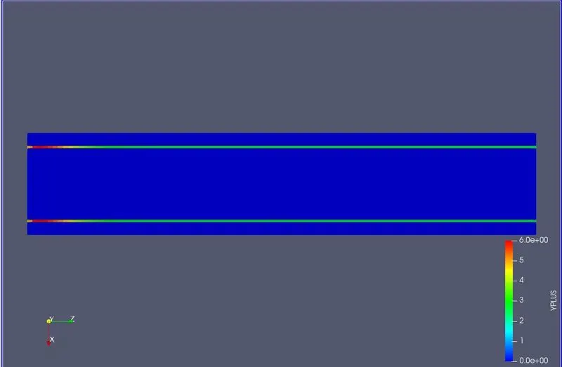
case 2:
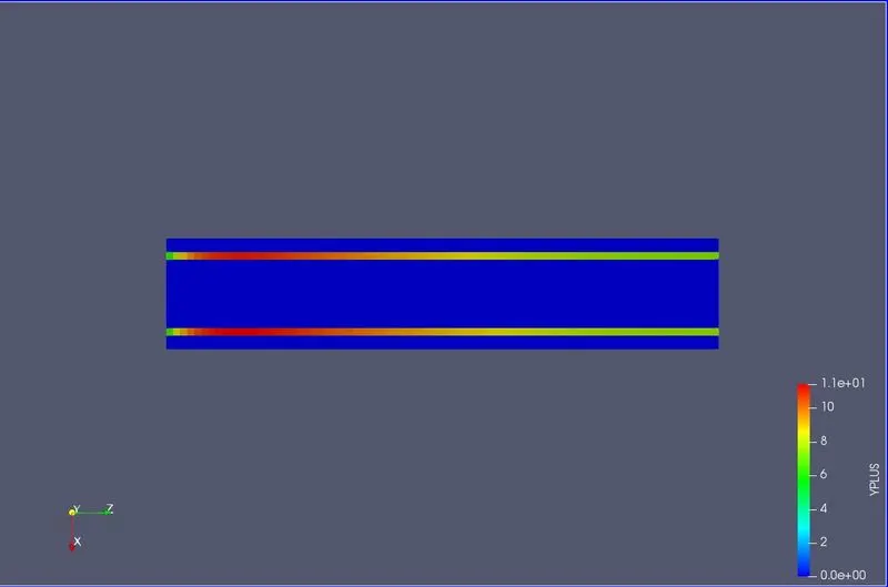
case 3:
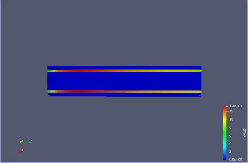
case 4:
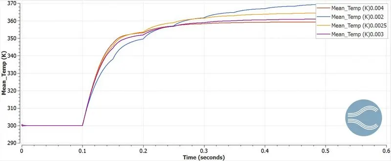
Mean Temperature Fluid Region:
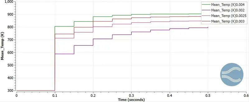
Mean Temperature Solid Region:
Total Number of Cells:
Super Cycle:
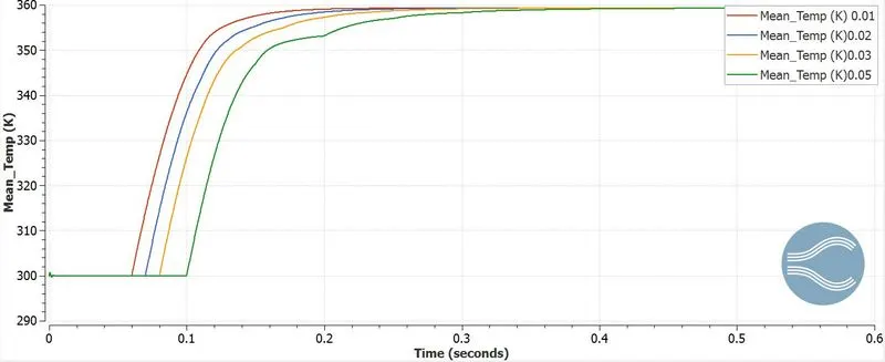
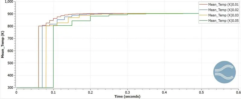
The concept of super charging is to pause the solid domain and solve the fluid domain initially.
Fluid Domain:
From the graph we can observe that when the super cycle stage is higher, the solution converges earlier.
Solid Domain:
From the graph we can observe that when the super cycle stage is higher, the solution converges earlier.
Super Cycle stage test:
|
Super cycle Stages mesh size 0.004 |
|||
|
SNo. |
Super Cycle stage |
Computation Time |
No. of cycles |
|
1 |
0.05 |
652.642307 sec |
2950 |
|
2 |
0.01 |
243.397225 sec |
3058 |
|
3 |
0.02 |
291.023031 sec |
3031 |
|
4 |
0.03 |
210.450485 sec |
3004 |
Conclusion:
- With respect to super cycling, we can observe that the computation time is lesser for lower super cycle stage values.
- Also the solution converges faster for higher super cycle stage values. This was infered from the mean temperature plots.
- It was found that smaller mesh values yielded better results.
Links to Animations:
Temperature:
Velocity:
pressure:
Y Plus