Conjugate Heat Transfer Simulation

Aim:

To setup a complete simulation of flow through a solid pipe with a constant heat flux applied to its outer surface.

Governing Equations:

The simulation is run on the basis of the Navier Stokes equations. The NS equation consists of three momenta, one continuity, and one energy equation. The energy equation is solved only during the time where there is a heat transfer taking place. This is done so to reduce unnecessary computational time.

Theory:

Conjugate heat transfer is basically a heat exchange between two different phases. Here, for example, the heat transfer is between solid and gas. To simulate heat transfer, three methods that include transient, steady-state, and super cycling methods can be used.

Transient heat transfer takes into account the path followed by the solid and gaseous phases during the heat exchange process. This would produce the ideal result but would be consuming a lot of computational time. As known with experience, solid bodies take a longer time to get heated up compared to a liquid or a gas. Hence, simulating the detailed path for the heat transfer of the solid would be very expensive computationally.

The steady-state solver would produce values at a faster rate, giving out the final steady-state values of the simulation. But since this does not include the path followed, the results obtained would not be faithful.

Super-cycling is a balance between the two. This would utilize both the steady-state solver as well as the transient solver. The way this solver works is listed out below.

• The solver would begin solving both the solid and gaseous phases together with the transient solver. After a specified cycle time, the solver would store the instantaneous Heat transfer coefficients and temperatures in the Interface.
• Once after a specified length of time, where the time can be an entire IC engine cycle or time required for complete flow through a body, the liquid side freezes, and the solid side is solved using a steady-state solver.
• Here again the time-averaged Heat transfer coefficients and temperatures and applies them as boundary conditions at the interface.
• The solver then updates all parameters and unfreezes the fluid side.

The cycle would run again up until the solid side reaches a steady-state value.

This type of solver would make sure that the values obtained are faithful while using as little a time as possible to obtain those results.

Case setup:

Before setting up the case, the boundaries were flagged as required. With one outside boundary where the heat flux was provided, one inlet boundary, one outflow boundary, one adiabatic wall between the inner and outer walls, and one interface boundary, a total of five boundaries were named.

Since the simulation involves both gaseous and solid materials, both docks were ticked with air being the material for the gaseous phase and Aluminium being the solid material. Global transport parameters were set to default numbers. Species were updated with the above-mentioned gaseous and solid phases. The run time was kept to be 0.8s with initial and minimum time step being 1e-7s.

Next, the regions were setup. Since again there were two materials, a solid-state region and a gaseous state region were created. The solid-state region was given a stream ID 1 with the solid check box ticked. Al was named as the species with a mass fraction of 1.0. The gaseous state region was set to steam ID 0 with the materials being the components of air i.e O2 and N2.

The Super cycling model was setup in the physical model block with the time length for each cycle stage varied between 0.01,0.02,0.03.

A grid size of 4mm was used initially and later was changed to obtain grid size based results. For the output variables, one another factor, y+ was also selected to later draw results from them.

Results and graphs

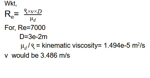
Before analyzing the results, the velocity for the inlet was calculated as follows:

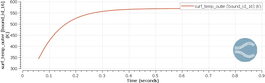
The surface temperature seen in the figure recognizes the increase in temperature of pipe with the addition of heat to its surface. The temperature rises at a slow rate reaching a steady-state value of 580K.

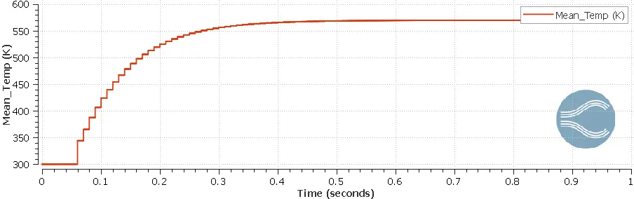
This value was confirmed by looking at the steady-state temperature of region 1 (solid) which also reached a value of 580K. The interesting observation is the step increase of the temperature curve at the beginning up until it reaches a steady-state value. These steps indicate the freezing and unfreezing of the gaseous phase during which the solid phase is simulated using a steady-state solver.

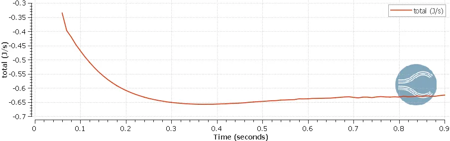
The total flux graph indicates the rate at which heat is transferred to the solid outer body with the curve showing s steady dip. This negative dip indicates the transfer of heat from surrounding to the system. The rate reaches a top rate of 0.65 J/s for around 0.1s as observed.

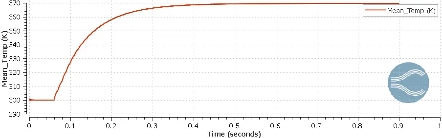
The next graph below shows the increase in temperature of the gaseous region that flows through the hot pipe. The graph initially stays at 300K for a duration of 0.1s where this time indicates the time required for heating of the solid pipe. Once after the pipe is heated enough, heat is convected to the air flowing through it increasing the temperature from 300K to 370K steady temperature as observed.

The other graphs below indicate the grid dependence test and the super cycling values changed from 0.01 through 0.03s.

Conclusion:

In conclusion, the simulation did run physically sound and produced faithful results indicating the setup was adequate. Also, reducing the supercycle stage interval time increases the simulation time but produces a converged result. The link for the youtube video would be https://youtu.be/mAUQF3H_H50