Emission characterization on a CAT3410 engine
Aim:
The project aims at obtaining emission characteristics of two different pistons, the open-w and omega pistons. The project further aims at drawing a comparison between the two.
Introduction:
Setting up a working engine initially requires importing a CAD file of the component from another environment to the CONVERGE studio. The CAD is then cleaned up by using the repair and patch options present in the software. This geometry was later flagged and the case set up was carried out step by step as mentioned in the coming sections.
Governing Equations:
The simulation is run on the basis of the Navier Stokes equations. The NS equation consists of three momenta, one continuity, and one energy equation. The energy equation is solved only during the time where there is a heat transfer taking place. This is done so to reduce unnecessary computational time.
Objective:
The objective is to obtain a sector surface for the diesel engine and later to set up a full hydro simulation.
The workflow involves:
- Importing the surface.dat file to extract bowl profile.
- Using the bowl profile to extract the sector geometry.
- Running the diagnosis to find out the errors in the geometry.
- Flagging the boundaries starting from the flow into the model and the fluid exiting from it.
- Creating the required case setup and setting up parameters according to the requirements.
- Transporting the input files and running the simulation.
- Convert the obtained 3D files into a corresponding viewable form.
- Obtaining the contours and animation and drawing results from them using a 3D viewing platform such as ParaView.
Case Setup:
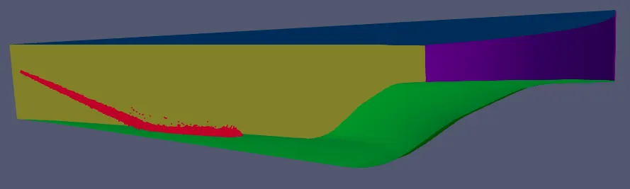
Before starting with the case setup, a sector geometry of the engine was created. Sector was created to be 60 degrees. It was done so to obviously increase the simulation time. To begin with, the surface.dat file was loaded to obtain the bowl profile of that particular piston. Later, the file that contained the bowl profile was loaded with the compression ratio fixed at 17.5 and the bore and stroke measurements provided accordingly. This process churns out a sector geometry of the engine with a sector angle of 60 degrees.
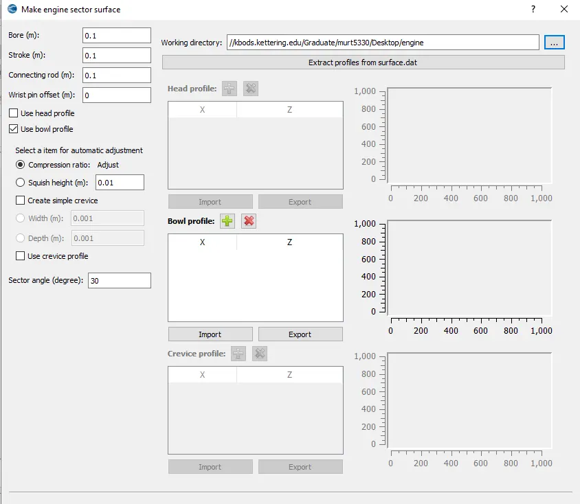
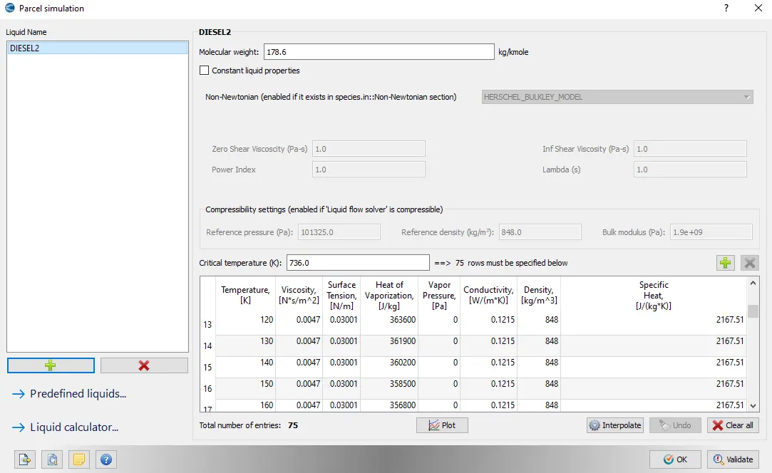
The application was chosen to be the IC engine. The boundaries were flagged. The flagged boundaries are as seen in . In the parcel simulation, diesel2 was selected to be the fuel with a molecular weight of 178.6 kg/kmole.
The simulation was set to run from -147 degrees to 135 degrees with a minimum time step of 1e-8 and an initial time step of 5e-7.
There was one cylinder region that was created and the species CO2, O2, H2O, and N2 were added as species.
Spray Modeling:
CONVERGE uses Lagrangian modeling or spray modeling for obtaining the spray sequence. For the gaseous solver, converge uses the Lagrangian solver and for the liquid sprays uses the Eulerian model. The fuel after getting sprayed in the engine experiences different kinds of forces. The fuel inside the engine is spherical shaped particles called parcels. These parcels after interacting with air present in the chamber break into primary and secondary parcels. Few other parcels collide with each other and form coalescence. Other parcels, due to the heat inside the chamber, evaporate into their gaseous form. A few other parcels experience the drop drag and lose their shape. The Lagrangian model takes into account all the above-mentioned forces experienced by the parcels. It also considers the effect due to turbulent dispersion.
The modeling is carried out in order to set up the injectors and the volume of spray coming out the injectors. The spray modeling required a detailed setup. In the general section, the parcel was chosen to be distributed throughout the cone. The turbulent distribution model was chosen to be the O’Rourke model since this model suits the gasoline-based simulation.
For the evaporation model, the source was chosen to be the base parcel species solved using the Frossling model. The source species was named to be C7H16. The liquid fuel mass fraction for calculating spray penetration was chosen to be 0.97. Which means the penetration length is 97% of the total length of the penetration. The distance measured is not the vertical distance but the distance along the axis of the injector.
The mass diffusivity constant was calculated using the below-mentioned formula
ρgasD=1.293D0Tgas273n0-1
The collision model was chosen to be the NTC collision model. Collision mesh was used to reduce grid sensitivity. This means that the parcels can now interact with parcels in not only their grid but across the grid. This helps in obtaining a more realistic model.
The interaction between the cylinder wall and parcels were chosen to have a wall film. This means that upon collision with the wall, the parcels would form a thin film on the surface.
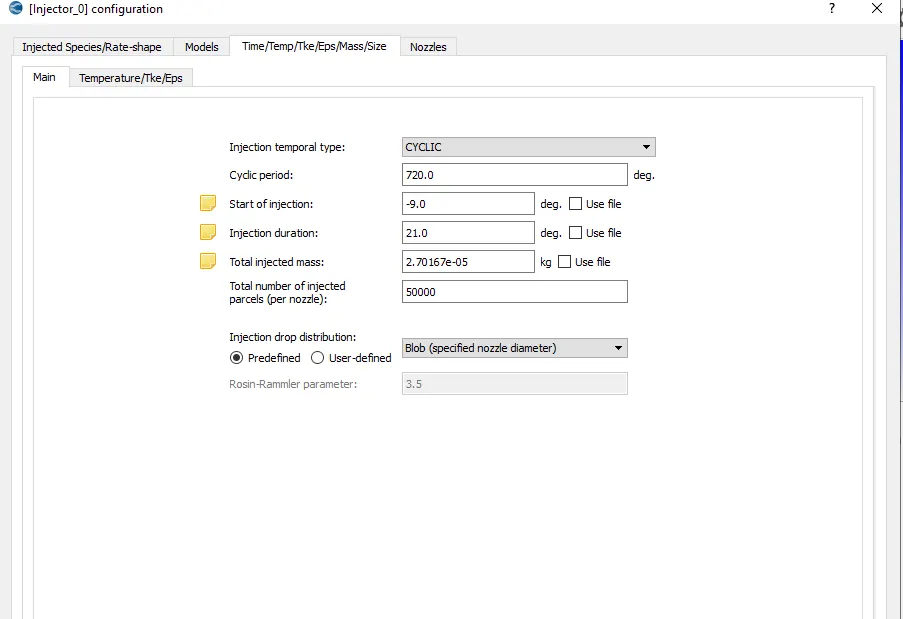
The injectors were set up as follows. The injector was chosen to have one nozzle. For the injection rate shape profile, points were drawn up the and the plot is as shown in the figure below. The parcel species was selected with a mass fraction of 1.
The injector was fitted with four nozzles each having a dia of 259μm and with a spray cone angle of 9 degrees. The injection start time was provided and a total of 27μkg of fuel was set to be injected.
Combustion Modeling:
For simulating the combustion, SAGE or the adaptive zoning model was utilized. The calculations of the model are based on the Arrhenius equations which are as given below.
kfr=ArTbe-ErRuT
Where,
Kfr is the forward reaction rate
Ar is the pre-exponential factor
b is the temperature exponent
Er is the activation energy
Ru is the universal gas constant
SAGE utilizes both the chemistry solver and the transport solver. The chemistry solver solves the rate of change of species(ODEs) and the transport solver uses the values from the chem solver as the source and uses it to obtain the change in species mass fraction during the length of the combustion.
Solving the chemistry side of the equations is computationally highly expensive since the solver has to produce the rate of change of each species of each cell. Hence to accelerate the process, there are a few things to consider.
To start with, a minimum temperature for the cell can be defined. Doing so would reduce the number of cells the solver has to go through. For complete combustion to take place, each cell should satisfy a minimum fraction of HC’s in them. Hence the solver allows defining a minimum mole fraction for each cell beyond which alone the solver can solve. Another easier solution is to provide a start time just before the start of combustion and end immediately after the combustion. The software also allows defining the solver to work only in certain regions. Since the simulation has to run multiple times, the cell whose temperature increases by a threshold factor can be provided. Another interesting solution is to combine cells to form bins. Bins can be based on two or more variables. This can help reduce computational time by asking the solver to go once per bin instead of once per cell.
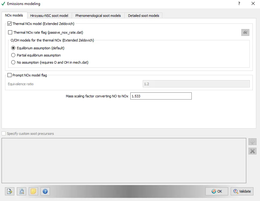
The emission model was checked along with the combustion modeling
Fixed embedding:
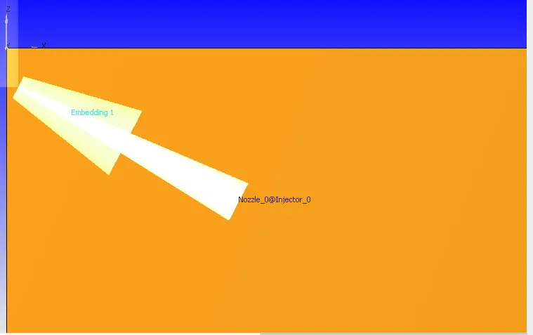
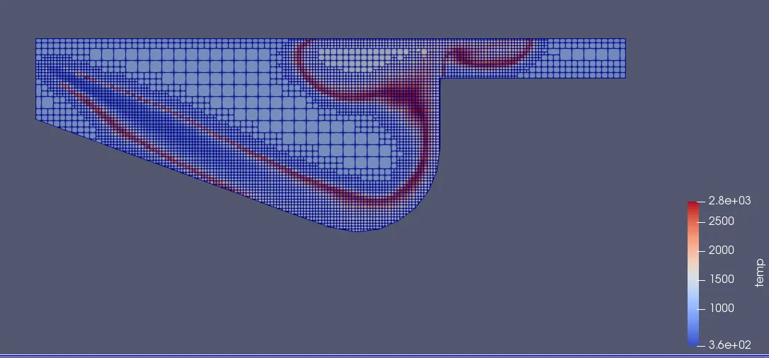
Embedding was carried around multiple parts of the engine. To capture the flow around the injector, cylinder head and nozzle, fixed embedding was created.
Adaptive Mesh Refinement:
The mesh refinement was provided to the cylinder and the intake port. The refinement was based on velocity and temperature with embed type being the sub grid scale. The Sub grid-scale was set to 3.
Regions and events:
The engine operation is cyclic with inlet and exhaust ports and other engine part’s opening and closing are in a particular sequence. These operations are replicated in the simulation using events. Events help in replicating the movement
The base grid size was chosen to be 4mm. The AMR was set up with the an embed level of 3 for both the velocity and temperature. This means that the smallest cell will be of the size
gridsize= basegrid/2embed-level
Results and graph:
The pressure plot for both the pistons show that open w piston has a peak of 11MPa compared to the 10.5MPa of the omega piston. This shows that the peak values of cylinder pressure are not much different.
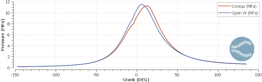
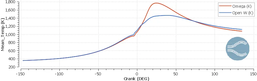
The peak temperature reched by omega piston is around 1700K whereas the open w reaches only around 1400K. The low temperature peak of the open w would mean that NOx levels would be down. But there’s another possibility where the low temperature can mean that the cylinder chamber contains unburnt fuel.
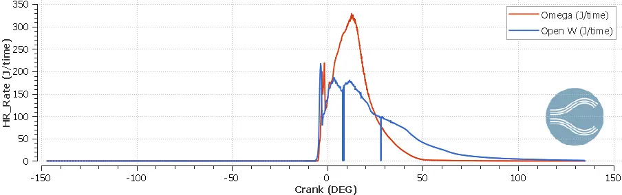
Heat release rate in J/time against the crank angle is shown below. A comparison shows that the omega piston reaches a peak of 330J whereas open w pistons only reach up to 200 J roughly. There is approximately 40% difference between the heat released between the two. This can be attributed to the peak temperature reached by the omega piston making them to release heat at a faster rate compared to the open w piston.
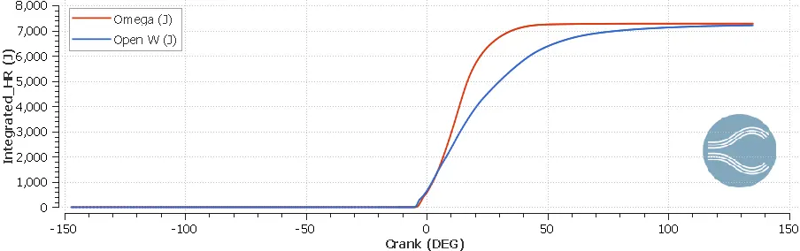
Integrated Heat release are results obtained by integrating the heat release over the entire cycle. This graph shows that the released heat rate is faster with the omega pistons compared to the open w pistons. There is a minute difference between the two steady states of around 50J between the two as can be seen from the graph. This difference actually is not quite small because the graph is integrated over one single cycle. If calculated over a range, say 1000 cycles, this difference is enormous.
To demonstrate, let us caculate the mass of fuel required for obtaining 50J of energy
Wkt, Q=mf*QHV*ηc
Here, QHV=42000 kJ/kg
ηc=0.98
Q=50J
mf=1.21μg
For around 1000 cycles, this mass would be 1.2mg of mass being used.
The NOx produced during the simulation of omega pistons is around 0.01kg, an 80% increase compared to the open w pistons. This can be attributed to the high temperatures and high rate of heat release that the cylinder chamber experiences. 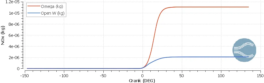
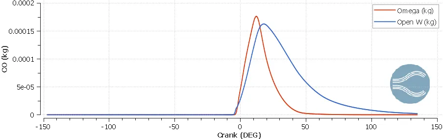
The CO produces implies there are unburnt fuel. Larger the amount of CO, larger the portion of the fuel that is left unburnt. Even though the omega piston has a peak higher than the open w piston, the open w produces CO for a crank angle larger than the omega piston. This can be attributed to not high enough peak temperature reached by the open w piston.
Now that the results have been studied, it can be concluded that open w pistons reach a lower peak temperature than the omega piston. A look into the spray injection shows the difference between the spray penetration into the cylinder before coming in contact with the piston. As seen, the omega pistons allow the injector to penetrate deep enough providing enough time for all the spray particles to get mixed with the air, eventually completing the combustion.
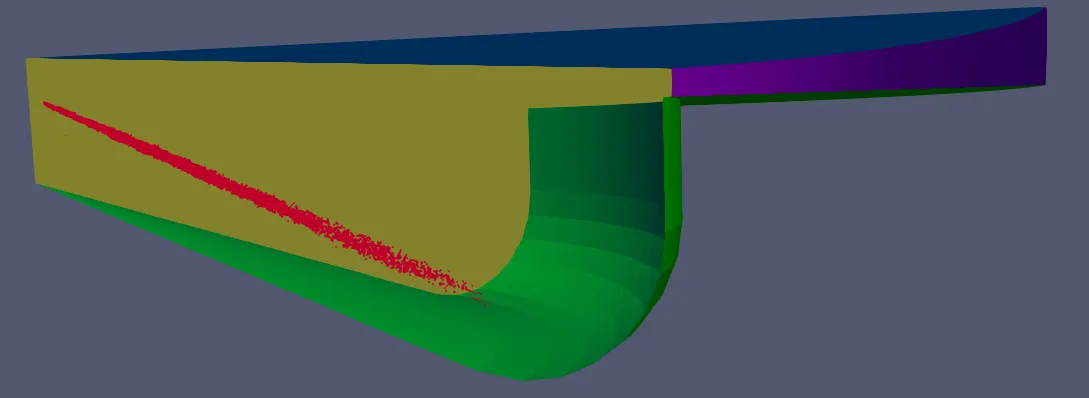
Whereas the open w piston, the spray does not penetrate enough impinging with the piston surface. This gives less time for the fuel to interact with the air molecules.
The fix to this can be utilizing the angle of injection. Changing the angle would make sure that the fuel can interact more with the hot air and more fuel can be combusted before impinging on the piston surface.
Engine performance:
The performance of both engines were compared starting with the power produced.
First the time required to complete the power stroke was calculated as follows:
The engine speed was considered to be 1600RPM
So that would mean a 26.66 rev per second
A revolution has 360 degrees in them and therefore 1600RPM would have 360*26.6 which gave 9600 degrees per second. This would mean that to rotate through a degree, it would take 1/9600 or 0.104 mili seconds. Hence it would require 0.104ms*270 (degrees of power stroke) equal to 28.08ms.
For omega piston:
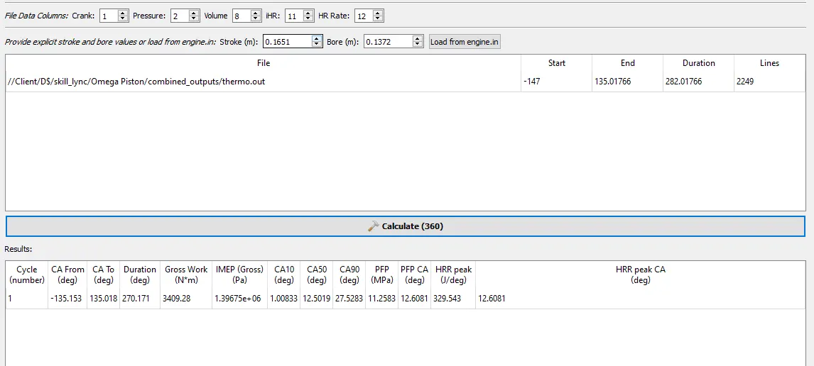
P=W/t=3409.28/0.02808=121.41 kW
For open w piston:
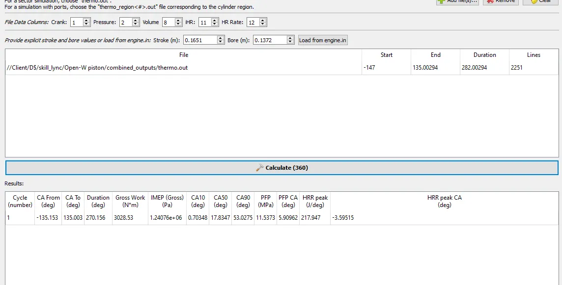
P=W/t=3028.53/0.02808=107.85kW
As seen from the above values, there is a significant drop in the performance of the open w engine. This is attributed to less work done due to low rate of heat release.
Looking at the CA10 values which means the crank angle at which 10% of the combustion is complete, the open w and omega pistons almost have similar values with open w reaching a bit slow.
The difference starts growing big which is confirmed by the CA50 values. The crank angle at which 50% of combustion gets completed is just 12 degrees after the top dead center whereas it takes 15 degrees to reach the same level.
The CA90 values clearly show the reason for the slow heat release rate as the open w takes a massive 53 degrees after TDC to reach there whereas the omega pistons take only 27 degrees, almost half the time required for the open w pistons.
Conclusions:
Overall both the piston were simulated effectively. Meaning that for both the simulations, piston’s movement and the exhaust gas obtained were captured faithfully.
If the engine is mainly used for reducing NOx emissions, then the open w piston works really well as observed in the discussions above. Apart from that, every other engine performance parameters are of a compromise.
The omega pistons provide a higher power output for the same input parameters. Hence considering the overall performance of the engine, omega pistons would serve the purpose.
But if the suggested correction with regards to injection angle of the open w is done, better performance can be achieved with them and might even produce output better than the omega pistons.