Week 6: Conjugate Heat Transfer Simulation
Introduction: Conjugate heat transfer is the method used to analyse the fluctuation of temperature within the solids and fluids. Heat transfers vary with respect to the medium i.e solid medium it takes place gradually due to its low capacitance and whereas In liquid it's faster due to higher heat capacitance. To attain steady-state temperature it takes more time. To eradicate this computational cost involved to attain steady, converge offers an alternative method called super cycling for overcoming this huge time which reduces the CHT simulation cost.
Case Setup:
Geometry and Mesh
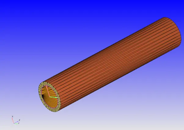
In this project above shown simple pipe with an inner diameter(orange) of 0.03, outer diameter(yellow) of 0.04 and length of 0.2(extended length -orange)) m is considered.
Mesh
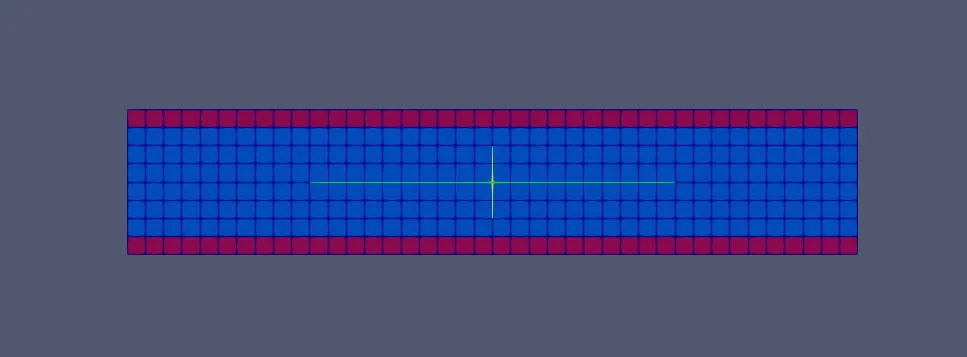
a) Grid - 4mm
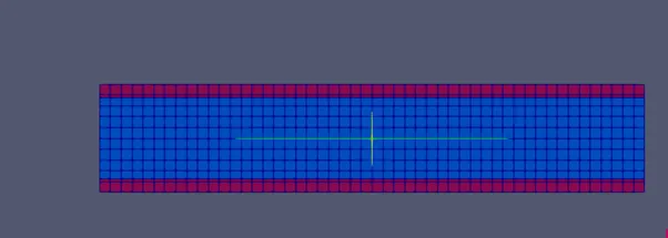
b) Grid - 4.5 mm
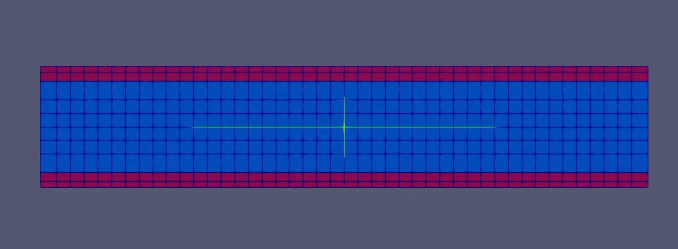
c) Grid - 5 mm
Boundary Conditions
The fluid used is the simulation is Air (O2+N2) and the solid material as Aluminium .Transient simulation is being set for 0.5sec .The turbulence model used in this is RNG k-epislon model.Below are the different boundary conditions considered for the geometry.
Inlet:
Boundary type: Inflow
Velocity:3.71 m/s(Based on Re=7000)
Temperature: 300K
Outlet :
Boundary type used here is outflow type with the pressure of 101325 Pa and backflow temperature is 300 K.
Solid side -Outer Wall:
The boundary type is a wall with a heat flux of -10000 W/m2
Interface between fluid and a solid domain:
Boundary type used is ''Interface'' with velocity formulation on the fluid side taking as ''Law of wall'' and solid side as Slip
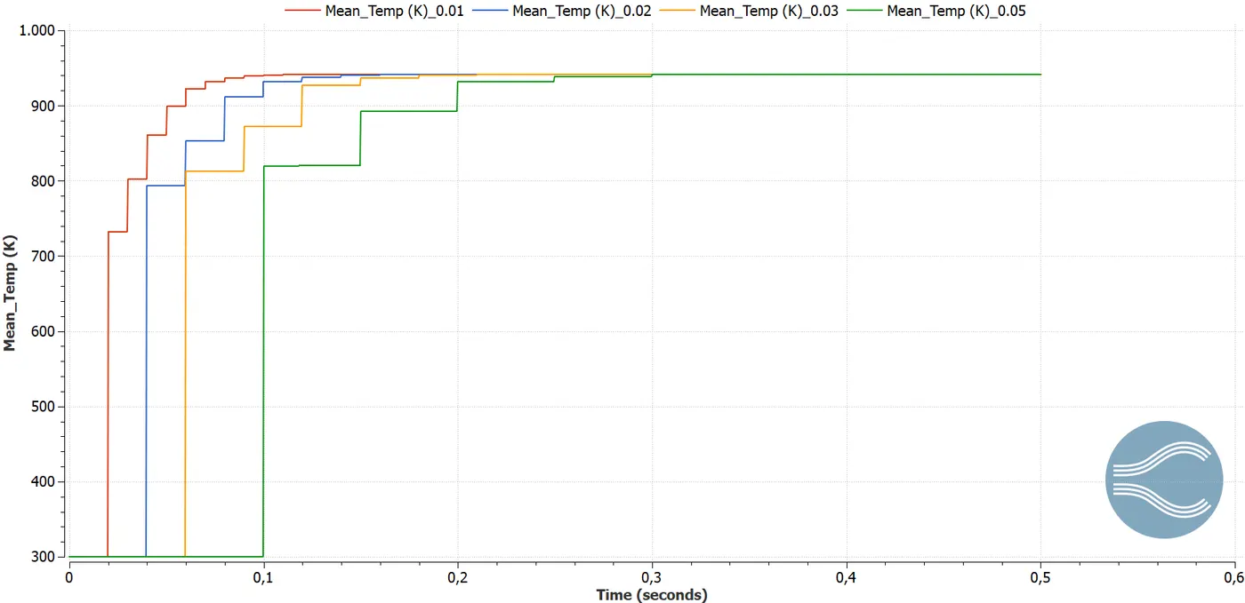
Along with boundary conditions, super cycling is applied with various super-cycle stage interval.In this simulation SCSI are 0.01, 0.02 and 0.03.
Results:
Grid dependency :
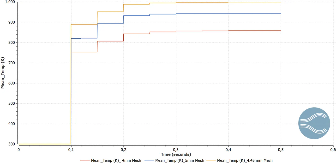
Based on the above temperature curve 5 mm mesh is used for further analysis of the supercycling effect.
Temperature for different Super cycling - 0.01
Contour Plots:
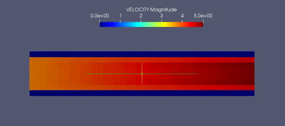
Supercyling - 0.01
Temperature:
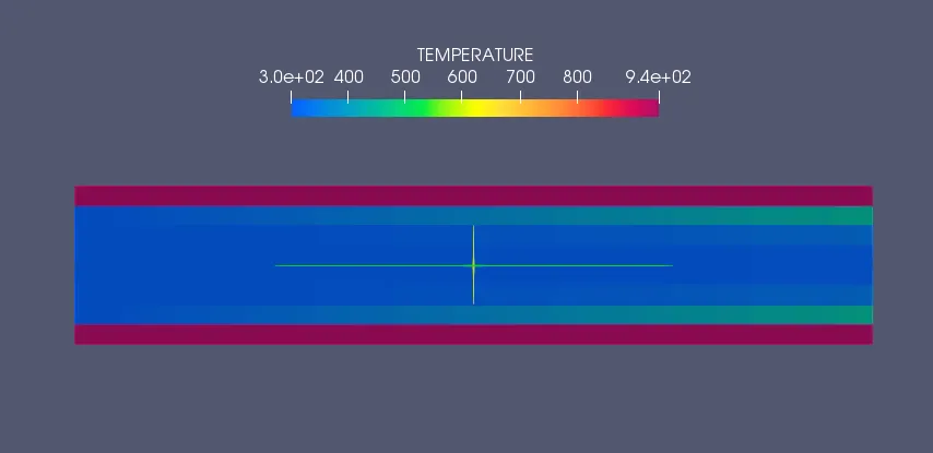
Below is the animation link
https://youtu.be/VXlmi8OPZgs
Velocity
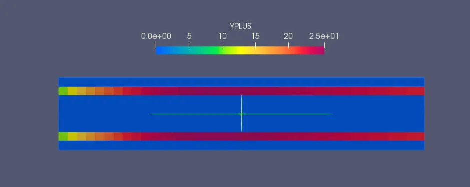
Yplus
Supercyling - 0.02
Temperature
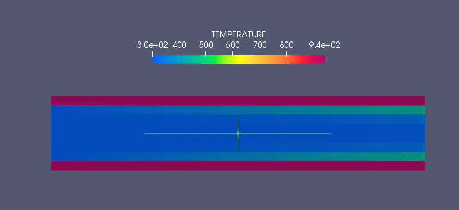
Below is the animation link
https://youtu.be/CM5-GiffYhw
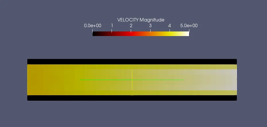
Velocity
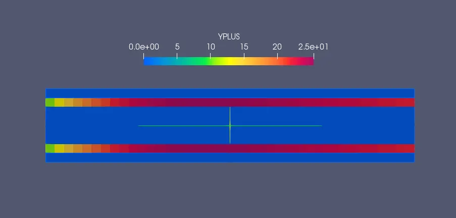
Yplus
Supercyling - 0.03
Temperature
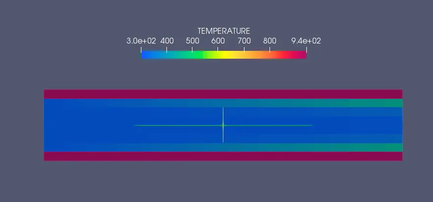
Below is the animation link
https://youtu.be/v3bkkXwOBgw
Velocity
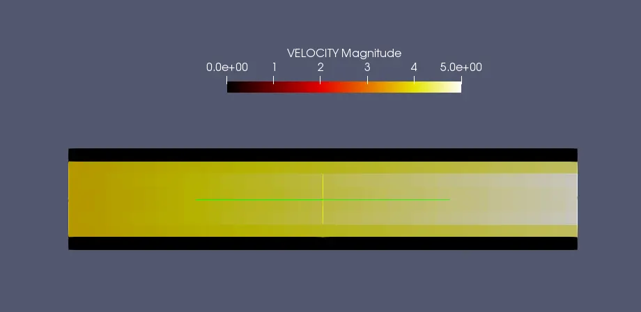
Yplus
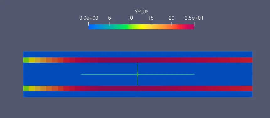
Conclusion:
To conclude, the temperature plots for the outlet indicates sharp increasing steps which depict the influence of super cycling effect until the temperature attains steady state. The maximum wall Yplus value observed is 25 which is constant for all three super cycling values as it depends on the grid size involved in the simulation. If grid size is further refined there is high chance of capturing detailed boundary layer phenomenon.Due to the application super cycling effect, solid domains reach steady state faster.