Week 6: Conjugate Heat Transfer Simulation

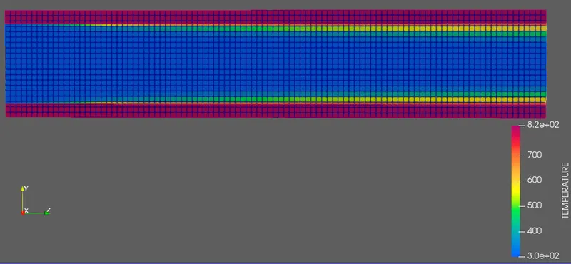
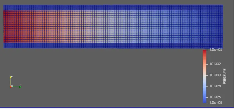
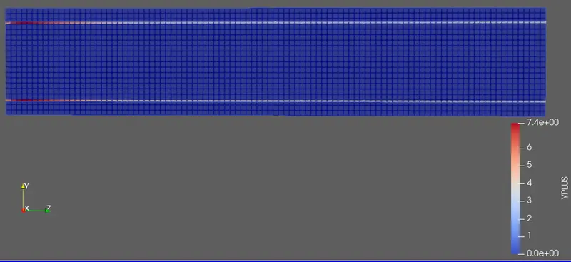
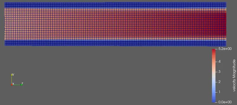
Aim:- Conjugate Heat Transfer Simulation

objective:-

• Setup a flow simulation through a pipe
• Inlet Reynolds number should be 7,000
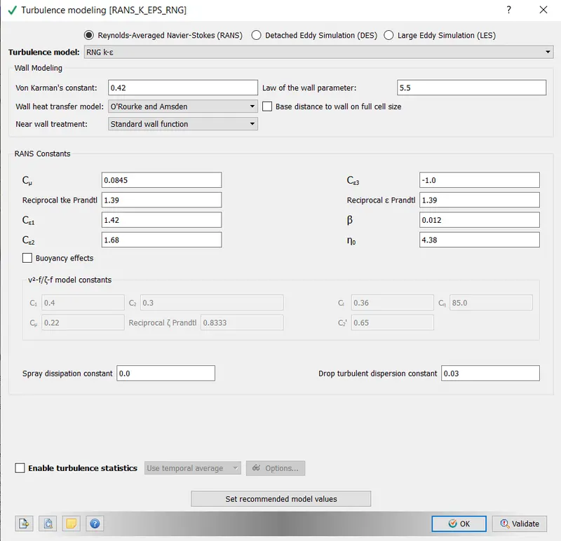
• Turbulence modelling - K-Epsilon
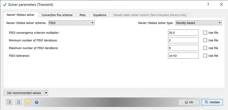
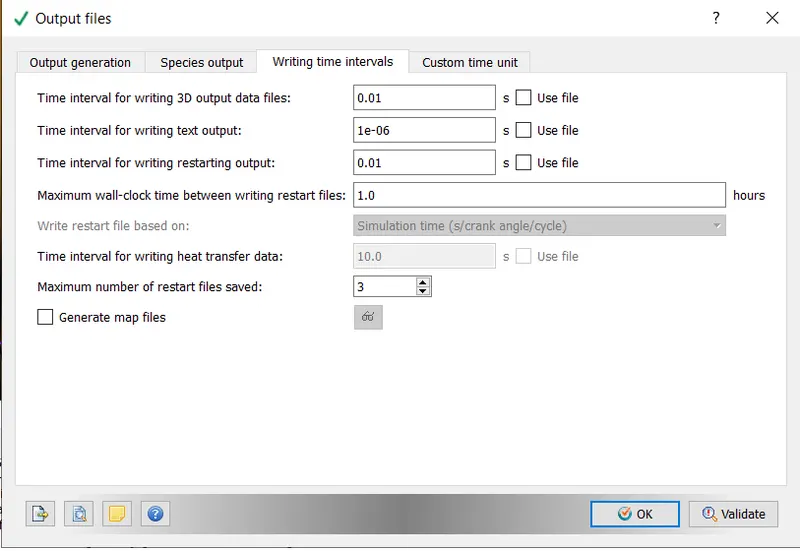
• Supercycling parameters

• Grid dependence test

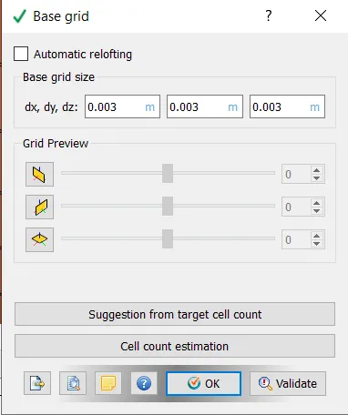
  • Start with an initial base grid
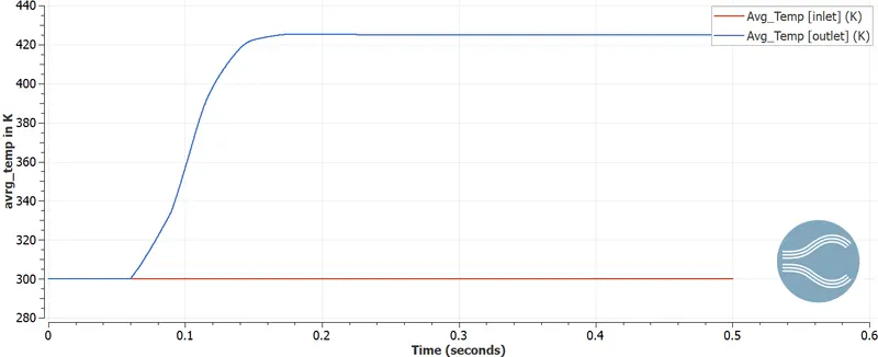
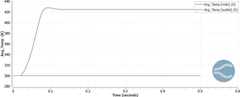
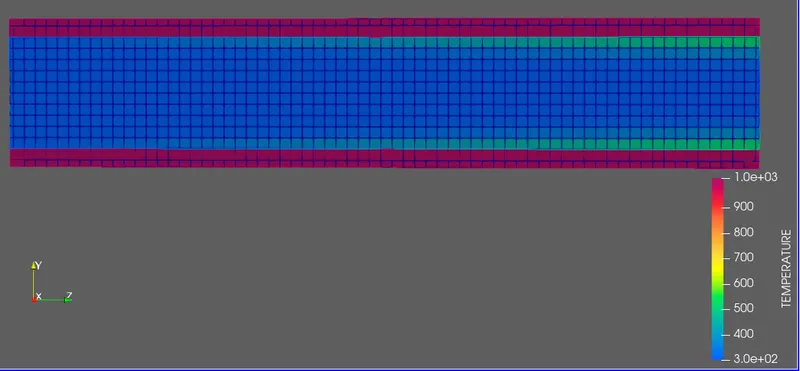
  • Run grid dependence test on 3 grids and show that the outlet temperature converges to a particular value

  Effect of supercycle stage interval

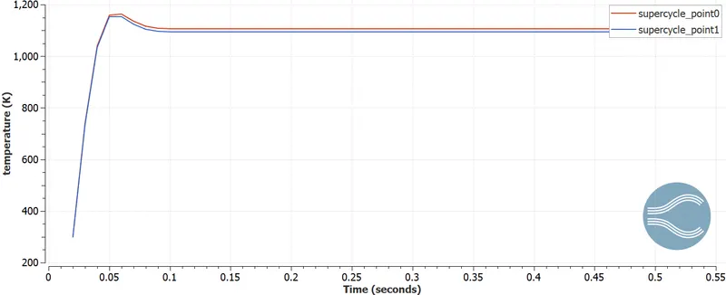
  • Set supercyle stage interval to 0.01,0.02 and 0.03

theory:-

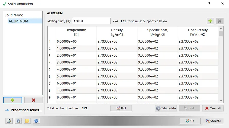
Conjugate Heat Transfer(CHT):-

Conjugate heat transfer corresponds with the combination of heat transfer in solids and heat transfer in fluids. In solids, conduction often dominates whereas in fluids, convection usually dominates. Conjugate heat transfer is observed in many situations. For example, heat sinks are optimized to combine heat transfer by conduction in the heat sink with the convection in the surrounding fluid.

Heat Transfer in a Solid:

heat transfer in solids, if only due to conduction, is described by Fourier’s law defining the conductive heat flux, q, proportional to the temperature gradient

`q=-k*gradT`

For a time-dependent problem, the temperature field in an immobile solid verifies the following form of the heat equation:

`rho*C_p(dT)/dt=grad*(k*gradT)+Q`

here Q is heat generation per volume if bogy generating heat

Heat Transfer in a Fluid

Due to the fluid motion, three contributions to the heat equation are included:

1. The transport of fluid implies energy transport too, which appears in the heat equation as the convective contribution. Depending on the thermal properties on the fluid and on the flow regime, either the convective or the conductive heat transfer can dominate.
2. The viscous effects of the fluid flow produce fluid heating. This term is often neglected, nevertheless, its contribution is noticeable for fast flow in viscous fluids.
3. As soon as a fluid density is temperature-dependent, a pressure work term contributes to the heat equation. This accounts for the well-known effect that, for example, compressing air produces heat.

Radiation: transfer of energy by electromagnetic waves between surfaces with different temperatures, separated by a medium that is at least partially transparent to the (infrared) radiation. Radiation is especially important at high temperatures, e.g. during combustion processes, but can also have a measurable effect at room temperatures.

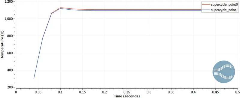
supercycle modling:

converge offer several time control methd for CHT in which supercycling is one option

here converge iterate b/w fully couple transient for fluid and stedy sate solustion for solid only

this method is highly recommend for combution simulation

during super cycling

1. intially solver solves fluid and solid using transient solver and store the heat transfer coeffient(HTC) and tepratuer on the interface during this precess
2. freezes the fluid solver: time avrging the HTCs and temp and applies them as boundary conction at the interface
3. solver the solid temp untilll it reaches steady state
4. update the solid temp field and unfreeze the flluid solver
5. repeat untill solid temp converge