Week 6: Conjugate Heat Transfer Simulation
Objective:-
To simulate the Conjugate Heat Transfer over pipe using Super- Cycling in CONVERGE and determine Y+
Theory :-
Conjugate Heat transfer (CHT) is when heat transfer occurs simultaneously within and between fluid and solid region
- The predominant mode of heat transfer in fluids is convection
- The predominant mode of heat transfer in solid is conduction
- CONVERGE solve the fluid heat transfer using the energy equation.
CHT is important for the study of
- Heat transfer from the engine block to coolant
- Engine block heating due to combustion
- Forced convection cooling of engine blocks
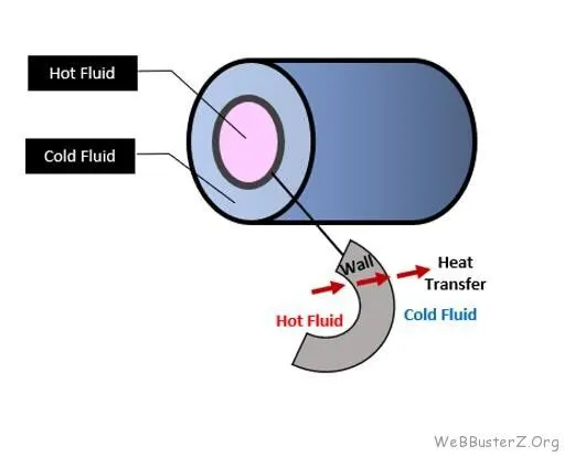
Super-Cycling Method:- In Super-Cycling method, the fluid solver working on convection problem is paused for a small time period allowing the solid state conduction solver catch up, this method significantly reduce the number of cycle and simulation time. Additionally, Super-cycling is a method used by CONVERGE Studio in the case of conjugate heat transfer problems with a solid and liquid regions.The integral problem here is that both solvers cannot run at the same speed since solving in the fluid domain is much faster owing to the time scale difference for heat transfer in liquids as compared to solids. This causes problems during the solution given that the solid side solver would not have reached a steady state/convergence in the time the liquid solver does. This is where the concept of super-cycling can be used.
Steps of Super-cycling
- Converge solves the fluid and solid together with the tansient solver and during this it stores instantaneous HTCs and temperature on the interface during this process
- It freezes the fluid solver and time-averages the HTCs and temperature and applies them as boundary conditions at the interface.
- Then it solves the solid temperature until it reaches steady-state
- It updates the solid temperature and unfreezes the fluid solver
- This process it repeats until the solid temperature converges
Applications:-
- It helps us to simulate & understand thermal systems like heat sinks,cooler,exhaust port of vehicle,HVAC,ICE etc.
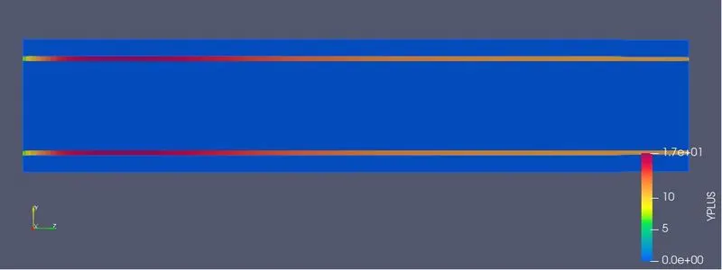
Output Y + :-
- Wall function are useful in telling the solver how to approch the solution near a wall. These used to predict near wall result accurately even at coarse grid.
- The Y + value is a non-dimensional term that can be used to understand how coarse grid are fine, this can then be used to determine if wall function need to be used or not.
For Calculation of Velocity:-
Reynold Number can be given as :-
Re=(ρ⋅v⋅d)/μ
where,
Re - Reynold's Numvber - 7000
ρ - density of air - 1.225 (kg)/m^3
v - velocity - to be calculate
d - diameter - 0.015 m
μ - 18.45 * 10 ^(-6) Pa.s (dynamic viscosity)
Therefore, Velocity can be calculated as
v=(Re⋅μ)/(ρ.d)
v = 7.028 m/s
Geometry : -
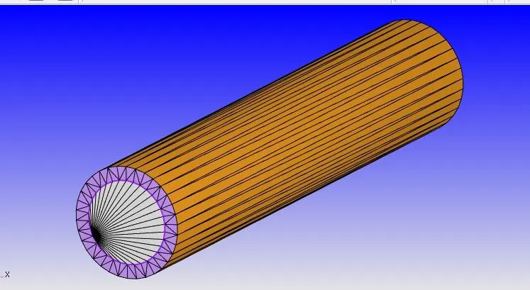
Geometry
Outer Diameter = 0.02 m
Inner Diameter = 0.015 m
Length = 0.2 m
CASE SETUP :-
Application type:-
- Time based
Material:-
- Gas simulation - Air
- Solid simulation - Aluminium
- Species - on
- Reaction Mechanism - off
Global Transport Parameter:-
- Turbulent Prandtl Number - 0.9
- Turbulent Schemidt Number - 0.78
Simulation Parameter:-
- Solver - Transient State Solver
Simulation time parameter:-
- Start time - 0.0
- End time - 0.5
- Initial time step - 1e-7
- Minimum time step - 1e-7
- Maximum time step - 1
Region and Initialization:-
1. Fluid Region:-
- Stream ID - 0
- Solid - OFF
- Temperature - 300 K
- Pressure - 101325 Pa
- Turbulent Kinetic Energy - 1
- Turbulent Dissipation - 100
- Species - Air - O2 - 0.23
- Species - Air - N2 - 0.77
2. Solid Region:-
- Stream ID - 1
- Solid - ON
- Temperature - 300 K
- Pressure - 101325 Pa
- Turbulent Kinetic Energy - 1
- Turbulent Dissipation - 100
- Species - Aluminium - 1
Boundary Condition:-
- Solid wall - Wall - Stationary - Slip - Heat Flux - (-10000 W/m2) (Solid Region)
- Solid side - Wall - ZNE (Solid Region)
- Inlet - Inflow - Pressure (ZNE) (Fluid Region)
- Inlet - Inflow - Velocity (DI) - z - 7.028 m/s - Species - Air (Fluid Region)
- Outlet - Outlflow - Pressure (DI) - 101325 Pa (Fluid Region)
- Interface - Interface - forward - Fluid region - Law of wall
- Interface - Interface - Reverse - Solid region - Slip - Aluminium
Physical Model:-
- Turbulance Model - k epsilion
- Super Cycle Model - Super cycle Interval - 0.05
- Super Cycle Model - CFL - 100
- Super Cycle Model - Relaxation - 1.4
Note - Go to post variable and check the yPlus section here in order to draw the graph in PARAVIEW.
Now, export the files to the destination folder and copy the 2 files such as Converge and mpiexe. from the C drive (where we installed Converge software) and put into the folder where we export the input files .
So Go to CYGWIN and Run the Simulation with the help of Commmand name " mpiexec.exe -n 3 converge.exe restricted "
Time at mesh 0.0015
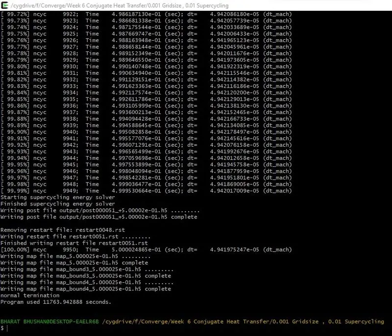
Time at mesh 0.002
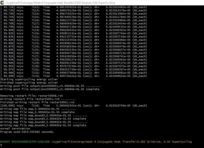
Time at mesh 0.003
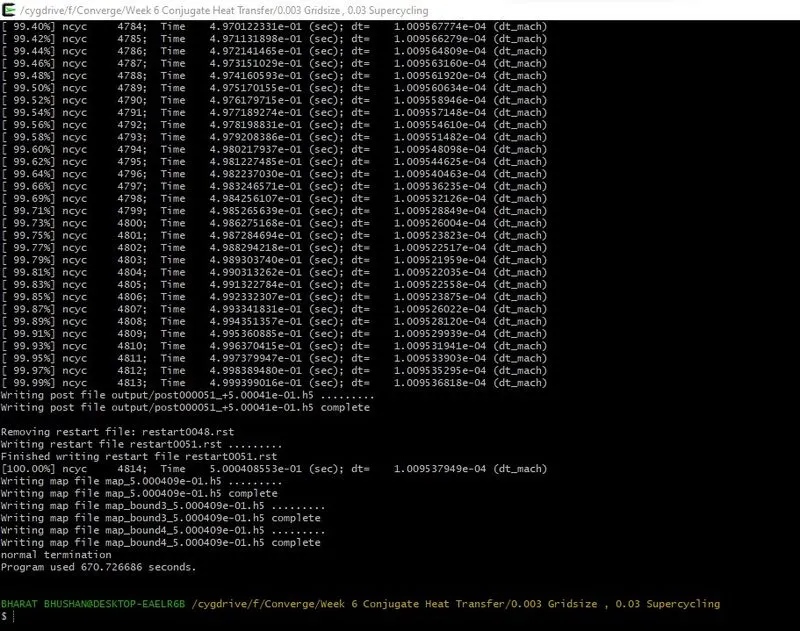
Time at BaseGrid Size mesh 0.01
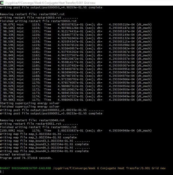
Table : Time(s)
Mesh
0.01 mesh (BASE SIZE) 74.371418
0.0015 mesh 11763.942888
0.002 mesh 5659.935682
0.003 mesh 670.726686
Again go to Converge and run the post processing as per given setup .
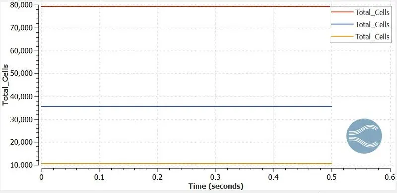
After completion of post processing left swipe click by mouse here we can see plotting window ,here plot the graph of Total cells as function of time as given below :
PLOTS :-
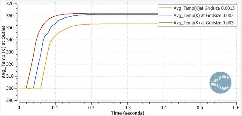
Average variation of temperature at Outlet:-
Cell Count : -
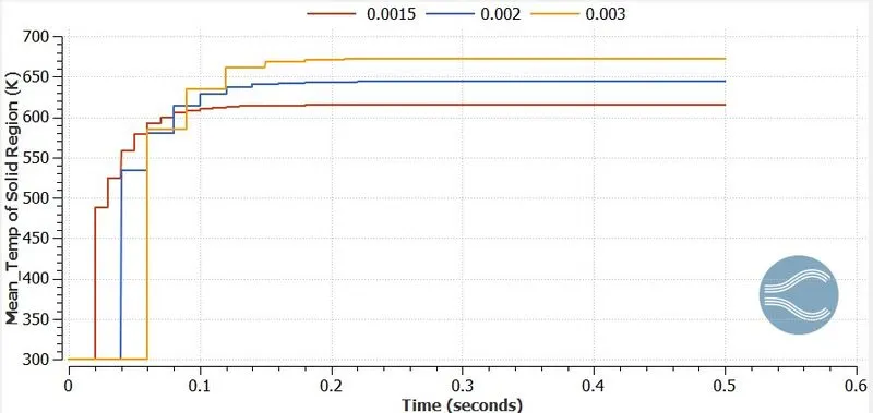
The steady state solver is employed in the solid region resulting in the sudden increase in temperature at various time intervals. This does not represent
the actual temperature flow in the solid and only the steady-state temperature. Note that the increase in the temperature in the solid regions is due to the heat flux added to the solid outer wall.
Mean Temp. of Fluid Region
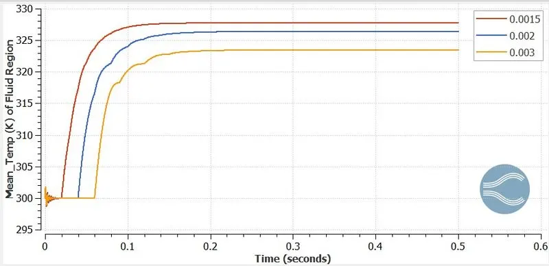
The transient solver is used to simulate the flow in the fluid region and hence the actual increase in the temperature is observed in this case. The increase in temperature is due to the
transfer of heat from the solid to the fluid.
Mean Temp. of Solid Region
SuperCycling Intervals of Time
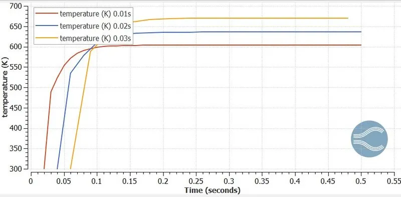
The time taken for the simulation for various value of supercycling time interval are as follows:-
| Supercycle stage interval | Temperature Value |
| 0.01 | 605.875 |
| 0.02 | 640.077 |
| 0.03 | 673.367 |
In the above reults, we set the different values of supercycle stage interval. The time length for each cycle stage from supercycling modelling to 0.01, 0.02 and 0.03. In the supercycling mode converge continue to solve both the fluid and solid equations and stores the heat transfer coefficient and near-wall fluid cell temperatures for a time equal to the supercycle stage interval. In the start converge solves both fluid and solid equations together using the transient solver (but does not store the solid heat transfer data ) from the start of the simulation until the supercycle start time in order to develop the fluid flow field. At supercycle start time converge begins storing values for a heat transfer coefficient and near wall temperature fpr each cell at the solid/fluid interface, one value for each time-step.
In the above plots, we can easily observe that setting the lower value of supercycle stage interval converges to the exact values of temperatures. Basically we increase the value of supercycle stage interval from 0.01 to 0.03. we got the more exact values at 0.03 supercycle stage interval.
In this part we performed the grid independency test with 0.0015m, 0.002m, 0.003m mesh size. By oberving the above plots we can easily say that at the finer mesh we got the more accurate values of temperature. But at the finer mesh computational effort has been increased.
Now, i will shift my mouse to PARAVIEW Application to launch Contour's and Animation's .
## PARAVIEW ##
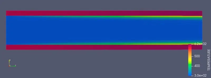
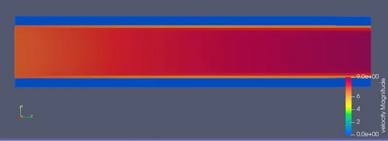
A. 0.0015 Gridsize and 0.01 SuperCycling
COUNTERS : -
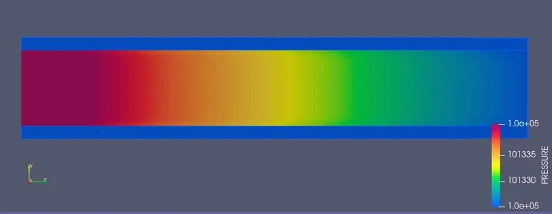
Pressure_Contour
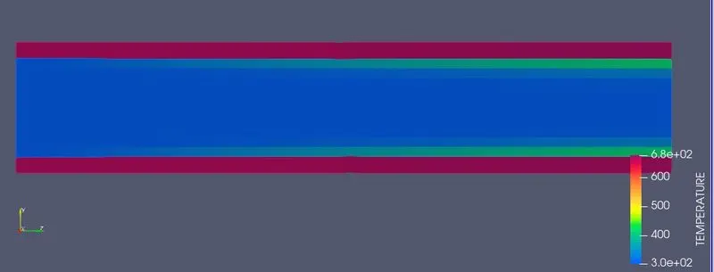
Temperature_Contour
Yplus_Contour
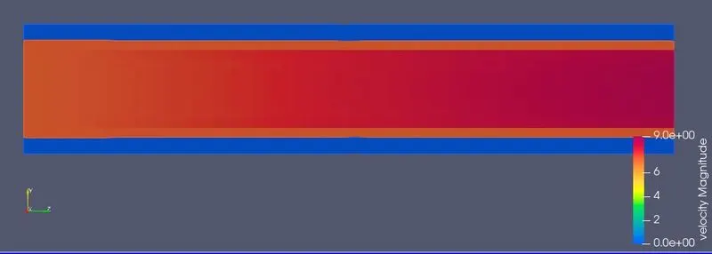
Velocity_Contour
ANIMATION :-
Pressure Animation
Temperature Animation
Velocity Animation
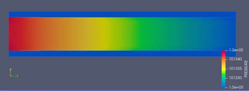
B. 0.002 Gridsize and 0.02 SuperCycling
Pressure_Contour
Temperature_Contour
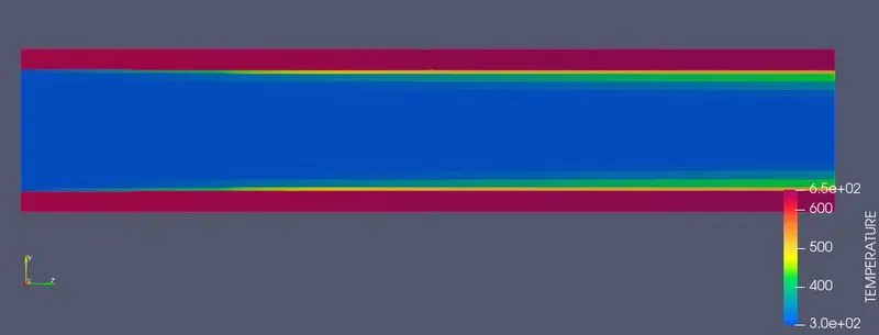
Yplus_Contour
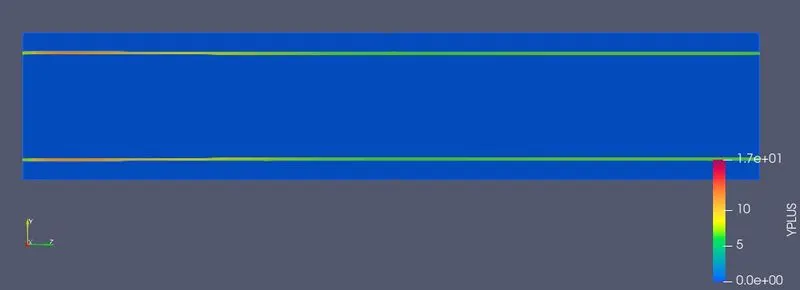
Velocity_Contour
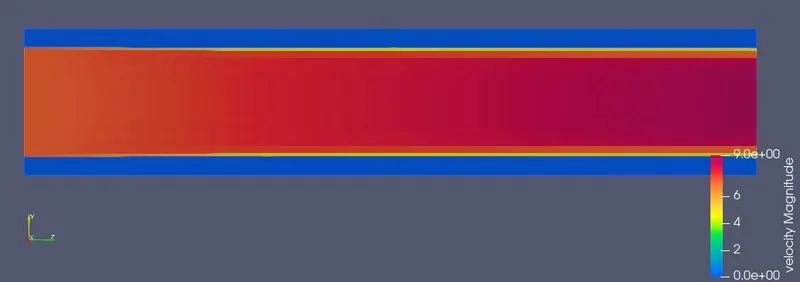
ANIMATION :-
Pressure Animation
Temperature Animation
Velocity Animation
C . 0.003 Gridsize and 0.03 SuperCycling
Pressure_Contour
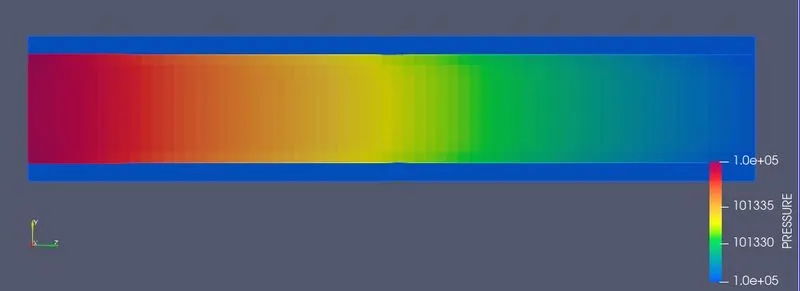
Temperature_Contour
Velocity_Contour
ANIMATION :-
Pressure Animation
Temperature Animation
Velocity Animation
C . 0.01 Baseline Mesh
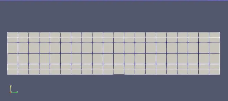
Mesh
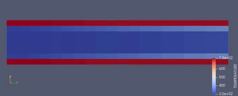
Temperature Contour
Velocity Contour
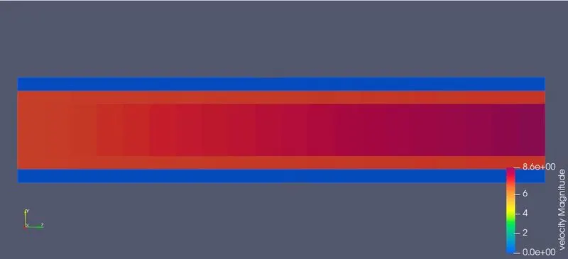
From the above figures we can see that the velocity at outlet is greater than the velocity at inlet. This is due to the decreased density at outlet, pressure at outlet also decreases and thus the velocity increases.
ANIMATION :-
Temperature Animation
Velocity Animation
CONCLUSION : -
- Transient conjugate heats transfer simulation of flow through a pipe is carried out for 0.5 seconds.
- The heat flux of 10000 W/m2 is applied on the solid outer wall and inlet velocity is calculated as 7.028 m/s based on the given Reynolds number 7000.
- Cut cell meshing strategy is used in converge studio. The total cell count for baseline, case 1 and case 2 are 343.612, 101811, 42951.4, and 12726.4 respectively..
- Contour shows that the pressure is high at the inlet and gradually reduces at the outlet to the specified in the outlet boundary conditions.
-
The heat flows from the outer wall to the inner wall of the pipe and then air picks up that heat and air gets heated increasing temperature higher on outer side and graduating reducing towards the centre of the pipe.
-
Grid Dependence:
In solid region: as grid refines solver predicts lower mean temperature.
In fluid region: as grid refines solver predicts higher temperature.
-
The convergence of graphs of different supercycling stage intervals shows at the end of the simulation all 3 cases converge at single-temperature shows the super cycling affects only time taken by the simulation to run not accuracy of final results.
- Studied super-cycling and Y+ plus and also their effect.
REFERENCES :
https://www.simscale.com/docs/analysis-types/conjugate-heat-transfer-analysis/