Week 6: Conjugate Heat Transfer Simulation
Objective:
To simulate the Conjugate Heat Transfer over pipe using Super- Cycling in CONVERGE and determine Y+
Theory:
Conjugate Heat Transfer:
Conjuate Heat Transfer correspond with the combination of heat transfer in solid and heat transfer in fluid.
• In solid, conduction often domain whereas in fluid convection usually domain.
Conjugate heat transfer is observed in many situation. For egs, heat sinks are optimized to combined heat transfer by conduction in the heat sink with the convection in the surrounding field.
Super-Cycling Method:
• In Super-Cycling method, the fluid solver working on convection problem is paused for a small time period allowing the solid state conduction solver catch up, this method significantly reduce the number of cycle and simulation time.
Output Y+:
• Wall function are useful in telling the solver how to approch the solution near a wall. These used to predict near wall result accurately even at coarse grid.
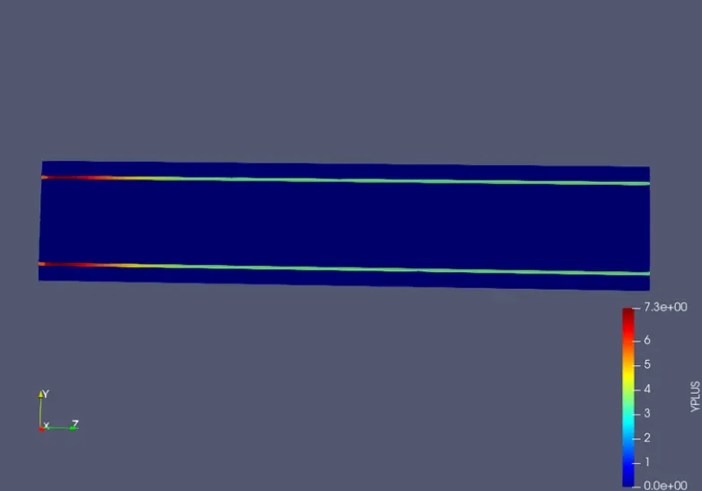
• The Y + value is a non-dimensional term that can be used to understand how coarse grid are fine, this can then be used to determine if wall function need to be used or not.
For Calculation of Velocity:
Reynold Number can be given as :
Re = (ρ*v*D)/μ
where,
Re-Reynold's Number - 7000
kg
ρ-density of air - 1.225 m3
v-velocity to be calculate
d diameter 0.015 m
μ-18.45 * 10 Pa.s (dynamic viscosity)
Therefore, Velocity can be calculated as
v=(Re*μ)/(ρ*D)
v=7000*18.45*10^-6
v = 7.028 m/s
Geometry:
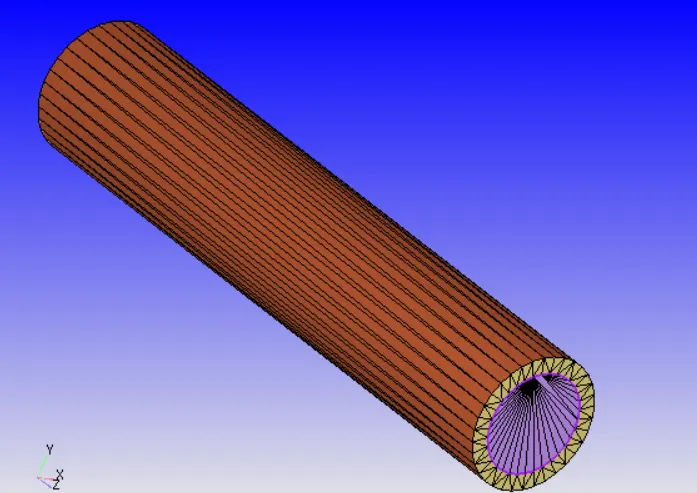
outer diameter=0.02m
inner diameter =0015m
length=0.2m
Case setup
Application type
Time based
Material:
1. Gas simulation - Air
2. Solid simulation - Aluminium
3. Species - on
4. Reaction Mechanism - off
Global Transport Parameter:
1. Turbulent Prandtl Number - 0.9
2. Turbulent Schemidt Number - 0.78
Simulation Parameter:
1. Solver Transient State Solver
Simulation time parameter:
1. Start time 0.0
2. End time - 0.5
3. Initial time step - le-7
4. Minimum time step - le-7
5. Maximum time step - 1
Region and Initialization:
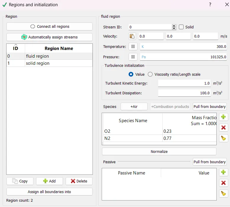
Boundary Condition:
1. Solid wall -Wall - Stationary - Slip - Heat Flux - (-10000 W/m2) (Solid Region)
2. Solid side - Wall - ZNE (Solid Region) 3. Inlet - Inflow - Pressure (ZNE) (Fluid Region)
4. Inlet - Inflow - Velocity (DI) - z - 7.028 m/s - Species - Air (Fluid Region)
5. Outlet - Outlflow - Pressure (DI) - 101325 Pa (Fluid Region)
6. Interface - Interface - forward - Fluid region - Law of wall
7. Interface - Interface - Reverse - Solid region - Slip - Aluminium
Physical Model:
1. Turbulance Model - k epsilion
2. Super Cycle Model - Super cycle Interval - 0.05
3. Super Cycle Model - CFL - 100
4. Super Cycle Model - Relaxation - 1.4
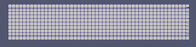
Case 1
for mesh size 0.004m
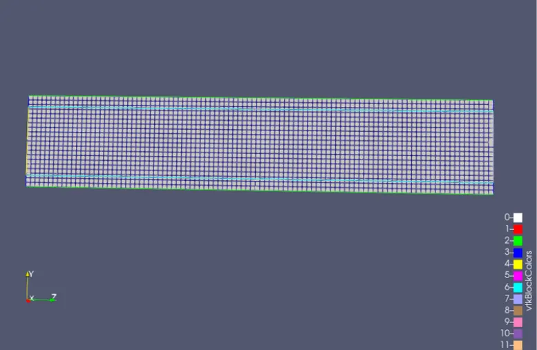
Mesh
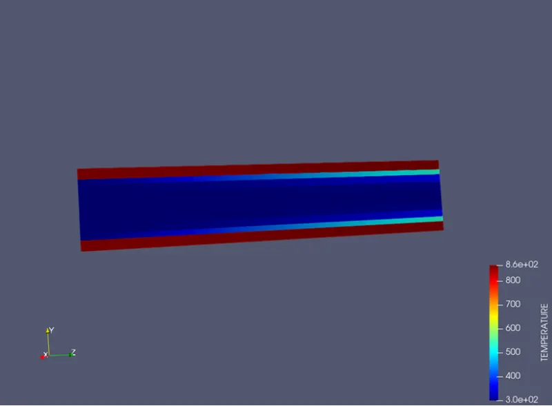
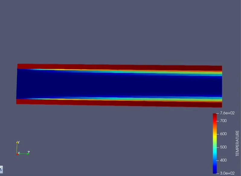
Temperature contour
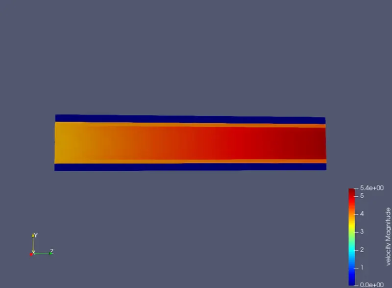
velocity contour
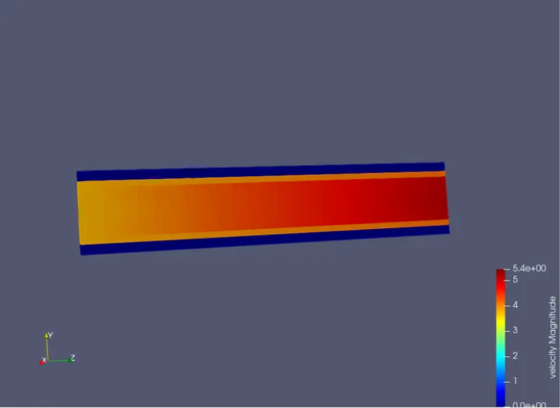
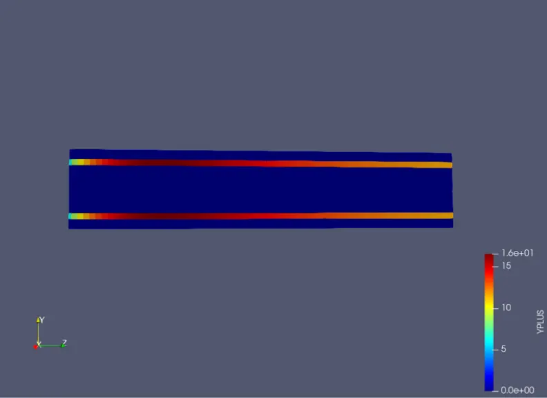
Y plus
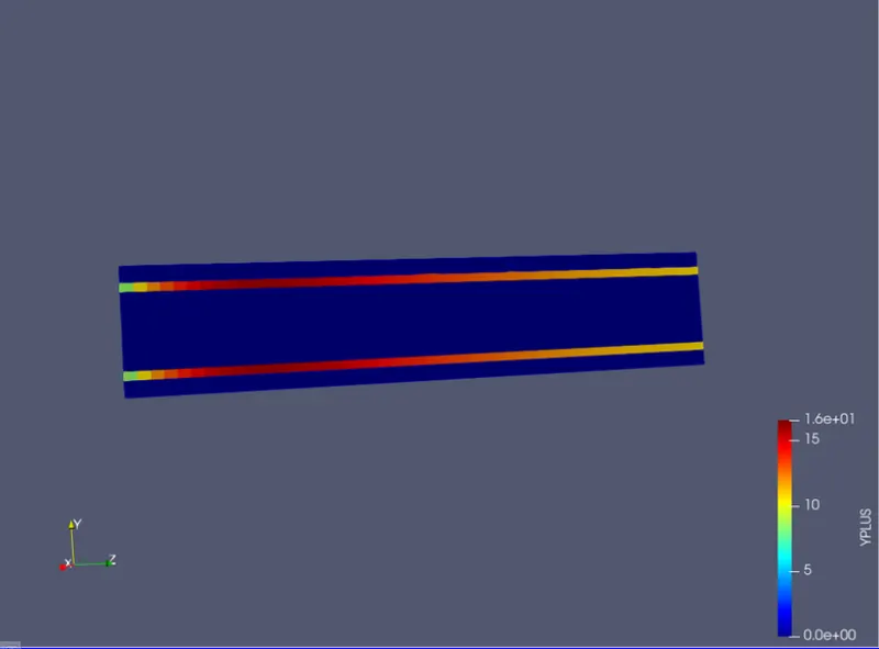
Case 2
for mesh size 0.003m
mesh
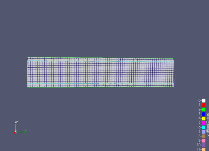
temperature contour
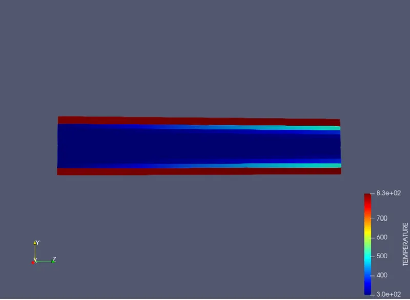
velocity contour
Y plus
Case 3
for mesh size 0.002m
mesh
temperature contour
velocity contour
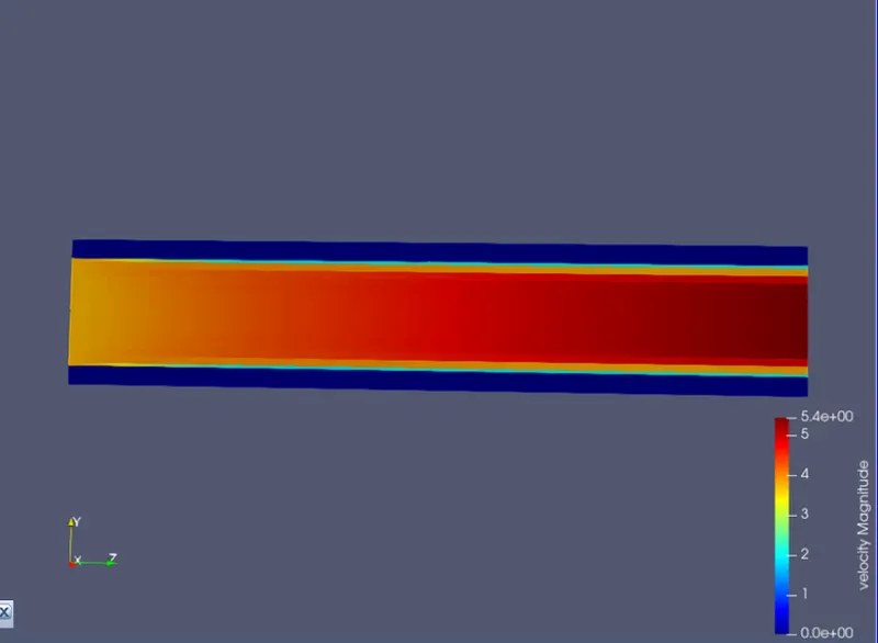
Y plus
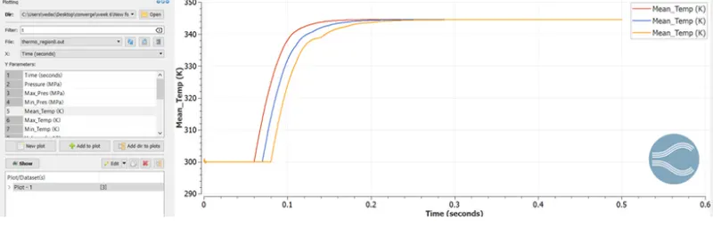
Fluid region
Solid region
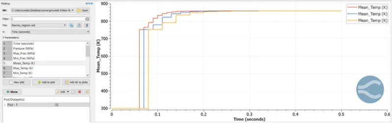
Based on super cycling
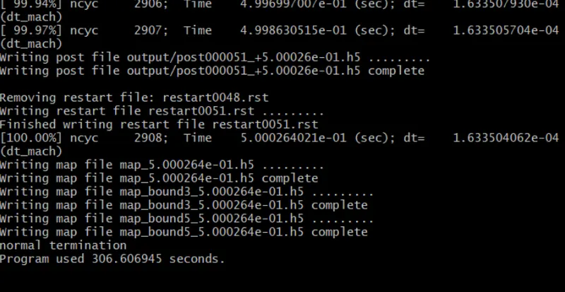
Case 1:0.01
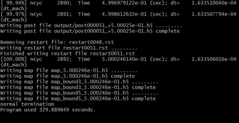
Case2 : 0.02
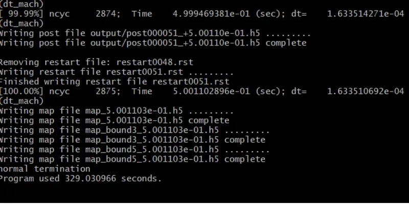
Case3 : 0.03
CONCLUSION:
- Refinement of grid results in clearer plots however at the expense of computational time
- Decreasing the SUpercycling time interval results in a reduction of computational time
- Irrespective of grid size, fluid values converge to a particular value.(380 K)