Week 6 - CHT Analysis on a Graphics card

Aim: To perform a steady state conjugate heat transfer analysis on a model of Graphics Card.

• Introduction:
• The term conjugate heat transfer (CHT) describes the process which involves variation of temperature within solids and fluids, due to thermal interaction between the solids and fluids, the exchange of thermal energy between the two physical bodies is called study of heat transfer, the rate of transferred heat is directly proportional to the temperature difference between the bodies.
• Conjugate heat transfer corresponds with the combination of heat transfer in solid and heat transfer in fluids, in solids, conduction often dominates whereas in fluids, convection usually dominates. efficiently combining heat transfer in fluids and solids is key to designing effective coolers, heaters or heat exchanger. forced convection is the most common way to achieve high heat transfer rate. in some applications the performances are further improved by combining convection with phase change.
• Heat transfer in solids and heat transfer in fluids are combined in the majority of applications. this is because fluids flow around solids or between solid walls and because solids are usually immersed in a fluid.
• Graphic card
• A graphics card (also called a video card, display card, graphics adapter, VGA card/VGA, video adapter, display adapter, or mistakenly GPU) is an expansion card which generates a feed of output images to a display device, such as a computer monitor. Graphics cards are sometimes called discrete or dedicated graphics cards to emphasize their distinction to integrated graphics.

Pre-processing :

Geometry setup:

• We have to Import the conjugate heat transfer (CHT) geometry file inside space claim.
• We have check is there any geometry cleanup needed or not.
• We have to go inside the work bench option.
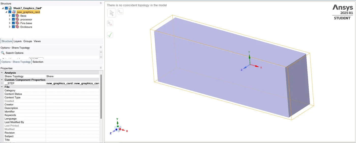
• We need to select the entire geometry and select the share option. Then check in Share topology by using this conjugate heat transfer (CHT) geometry can share information.

Mesh setup :

• We have go inside mesh in Ansys fluent.
• We have to generate mesh with Baseline mesh and Refined mesh.

Baseline mesh

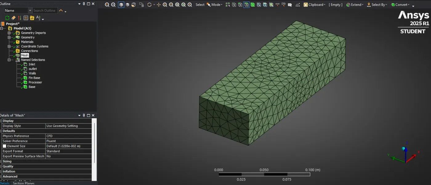
• We have to take by default element size in baseline mesh.

Refined mesh

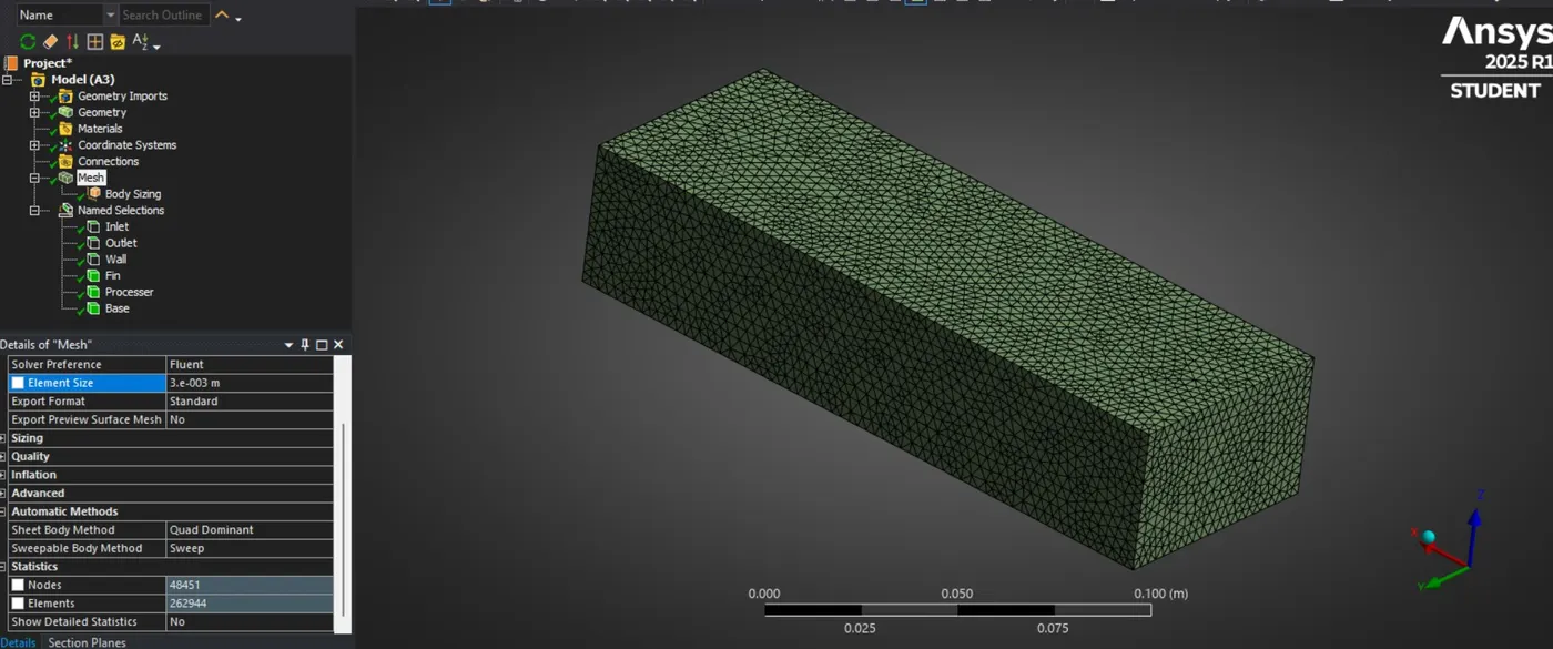
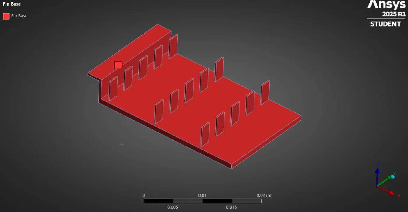
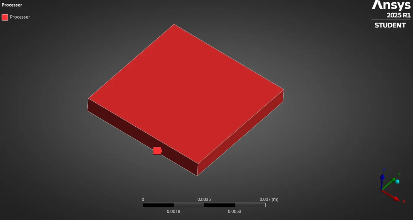
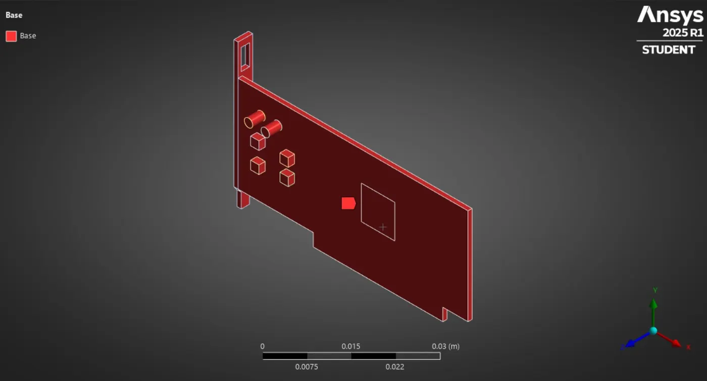
• We have to take element size is 0.002 m which is Fin , Base and Processer.

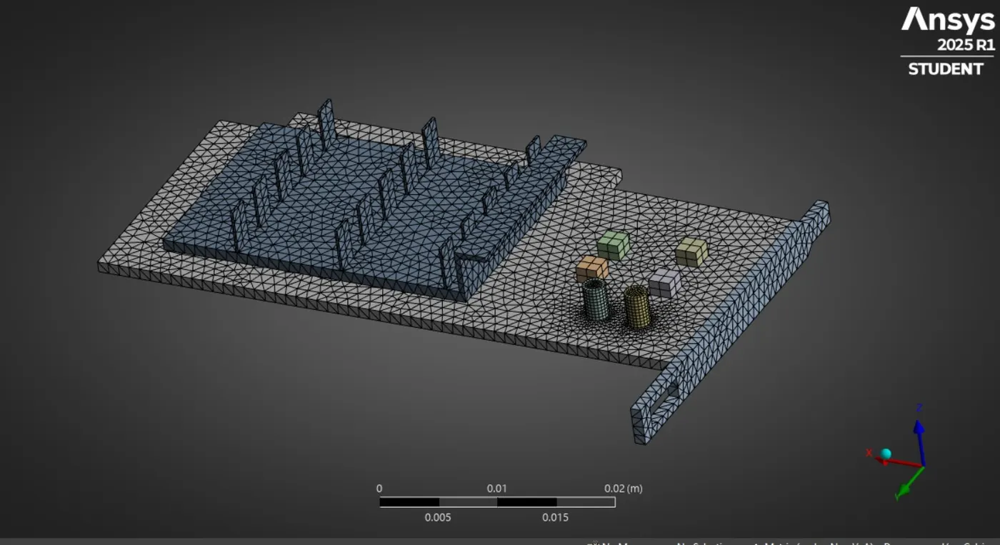
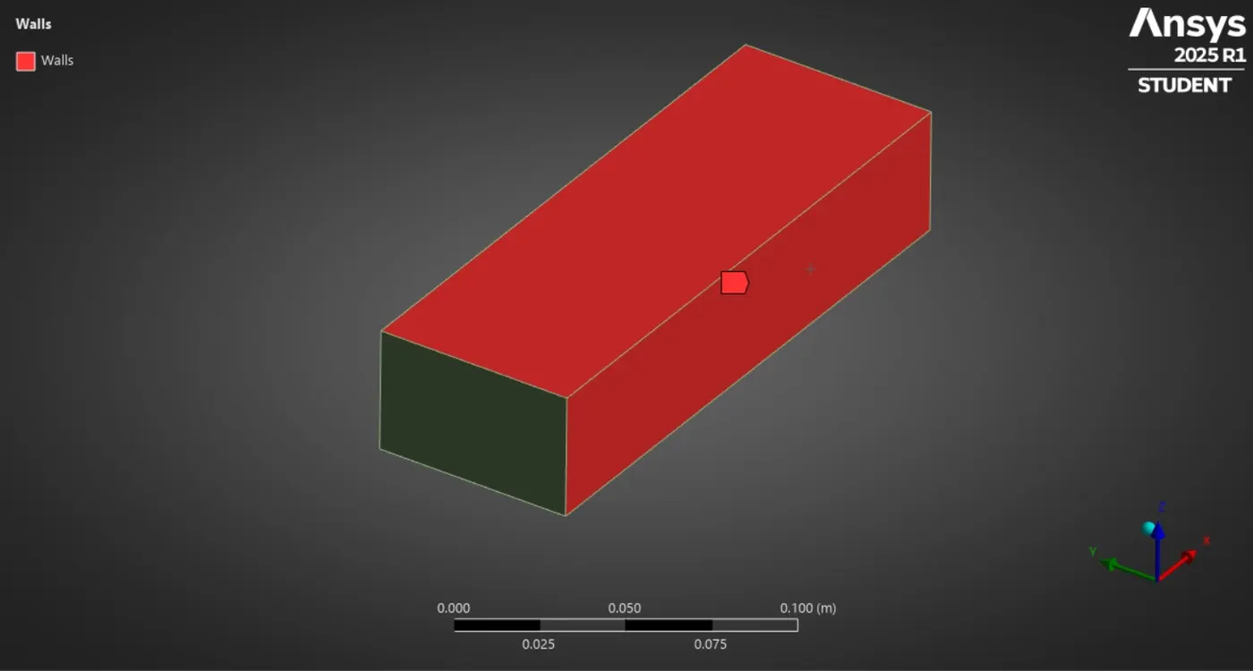
• We have to create name selection which is Fin , Processer , Base , Wall , Inlet and Outlet.

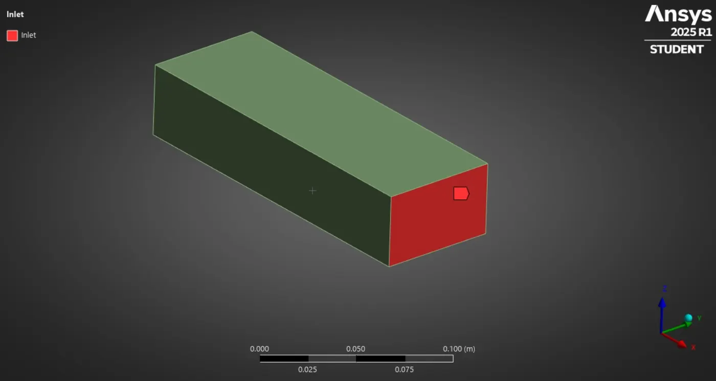
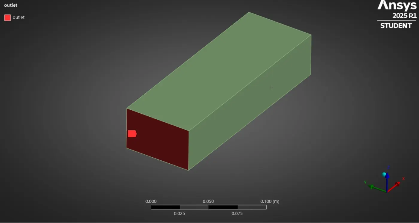
Fluent setup :

• We have to click on pressure based solver and also we have run with steady state solver.
• We have to go inside physics and select the energy option.
• We have to take K-epsilon inside the viscous (Turbulence) model.

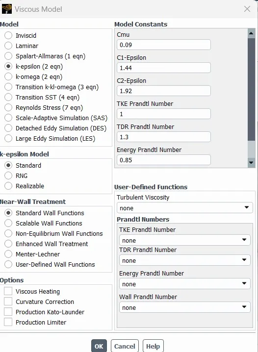
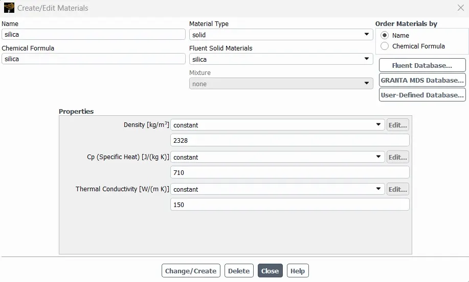
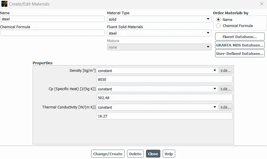
• We have to create materials which is Silica , copper and steel .

Silica ( Processer )

Copper ( Fin )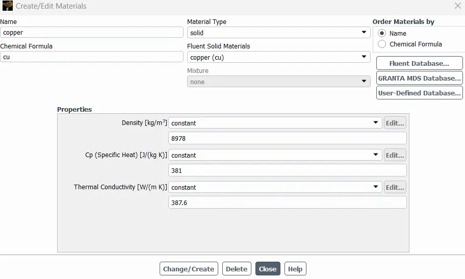

Steel ( Base )

• We have to go inside cell zones.
• Inside cell zones we have to change the material type which is solid , its like ( Silica for Processer , Copper for fin and Steel for base ).

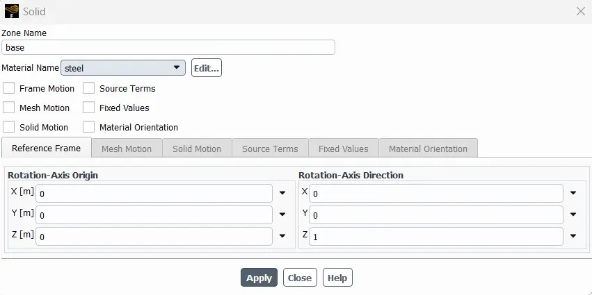
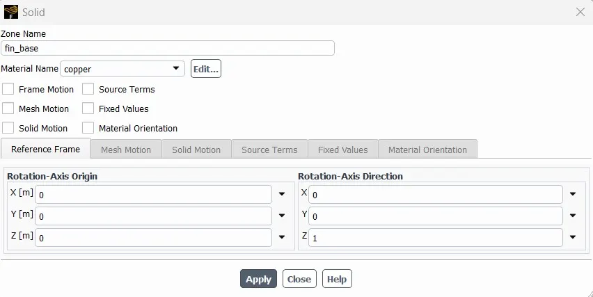
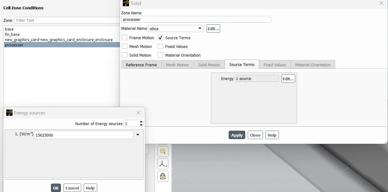
• We have to a energy source inside processer because from processer temperature are generates in every second in real life. Then we are going to calculate to give the value inside the energy source.

1. Heat generated Volume = Q / Volume
2. Q = 1 watt
3. Volume of processer = 64 mm^3
4. Heat generated rate = 1*10^9/ 64 = 15625000 w/m^3

Baseline mesh simulation

Case-1

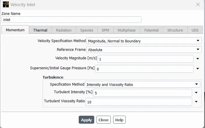
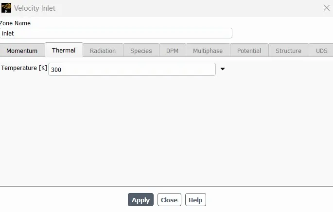
• We have go inside the boundaries then click on inlet .
• First we have to give the velocity magnitude is 1 m/sec .

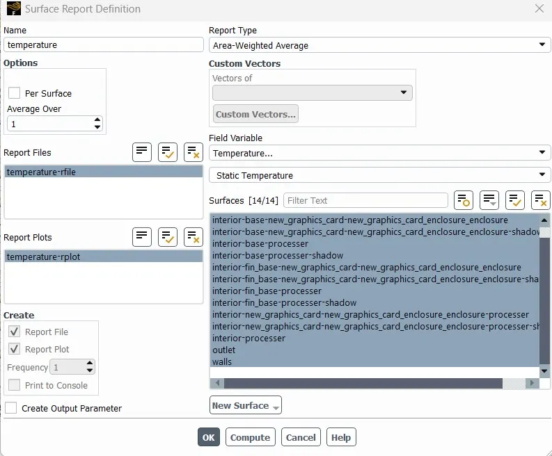
• We have to create a Temperature and Heat transfer coefficient plot inside the definition.

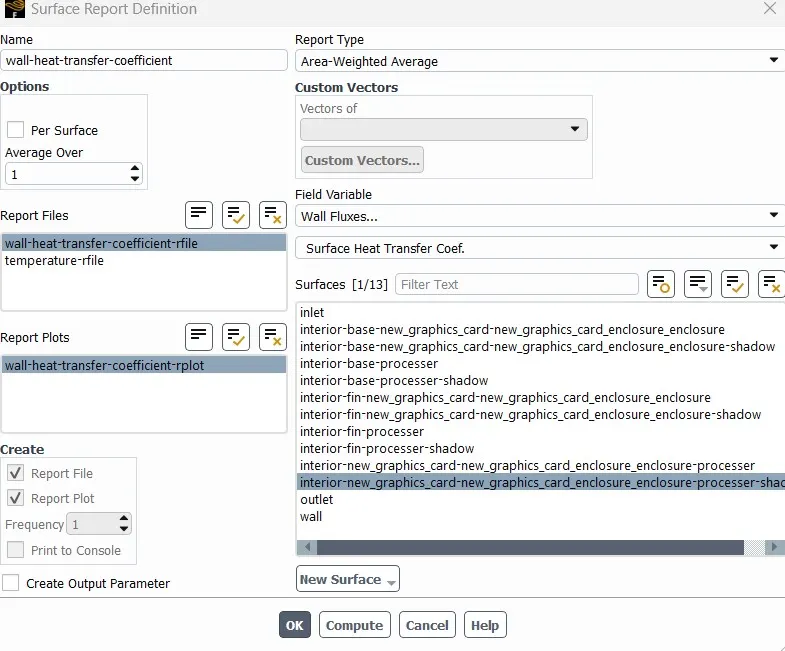
• Then we have to initialize the model.
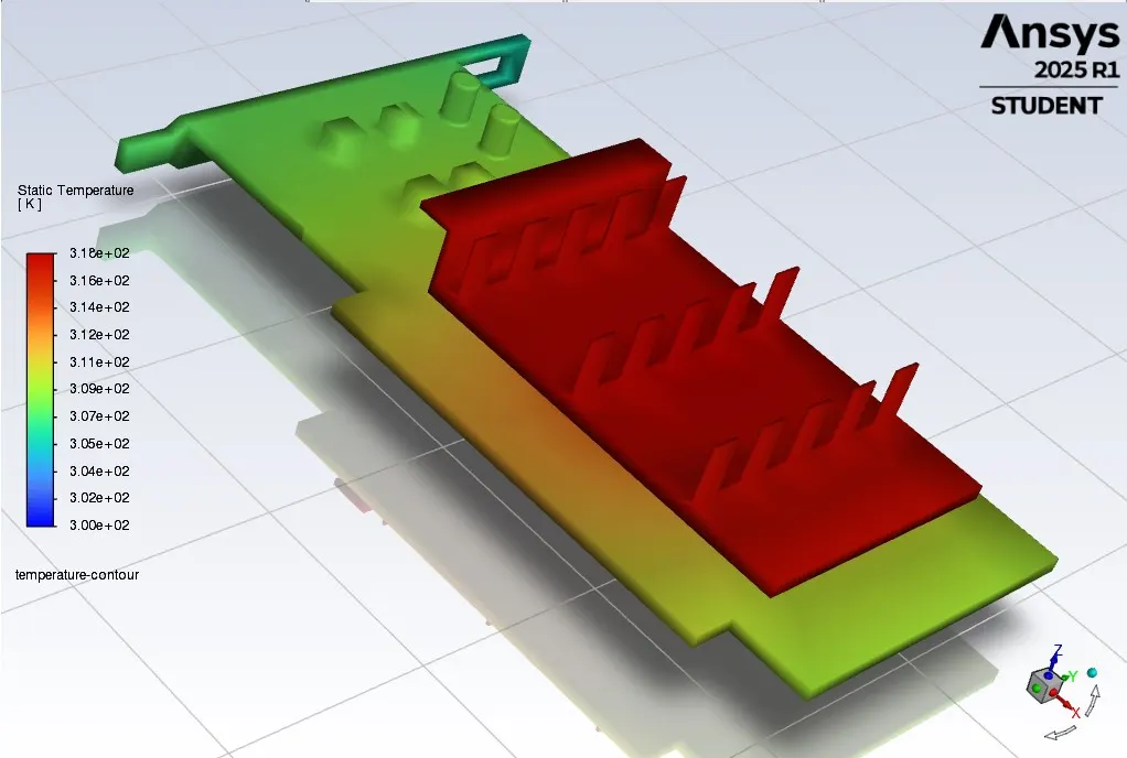
• We have to create a temperature contour plot.
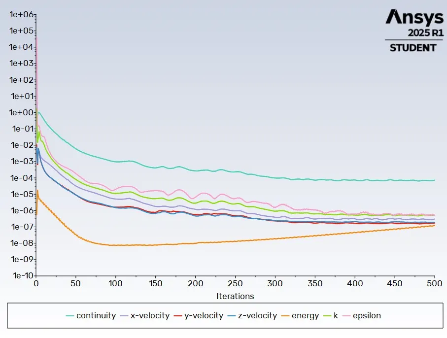
• We have to calculated the 500 time iterations.

Temperature contour ( 1 m/sec ):

Residual Plot ( 1 m/sec ):

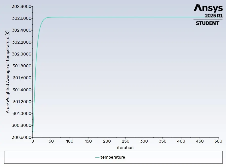
Temperature plot ( 1 m/sec ):

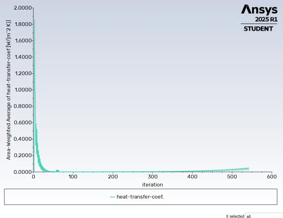
Heat transfer coefficient ( 1 m/sec ):

Case-2 :

• Again we have go inside the boundaries then click on inlet .

• We have to give the velocity magnitude is 3 m/sec .

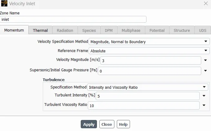
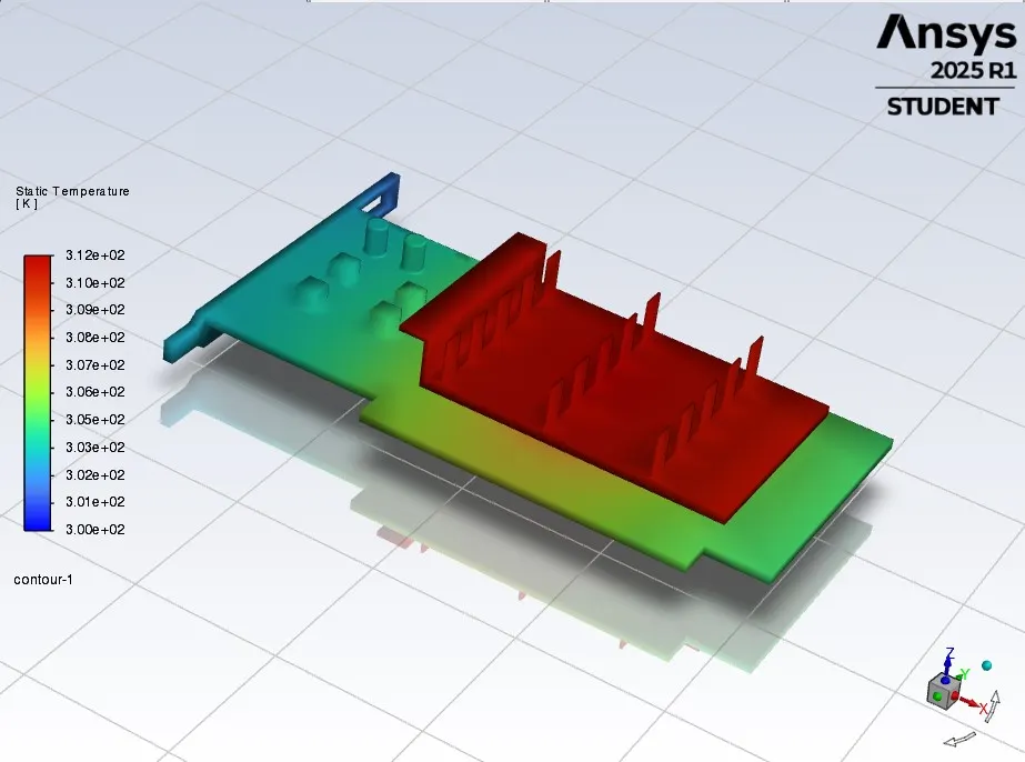
Temperature contour ( 3 m/sec ):

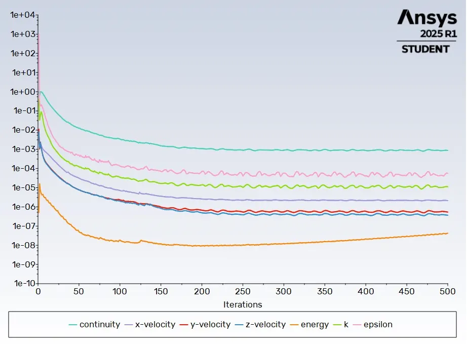
Residual Plot ( 3 m/sec ):

Temperature plot ( 3 m/sec ):

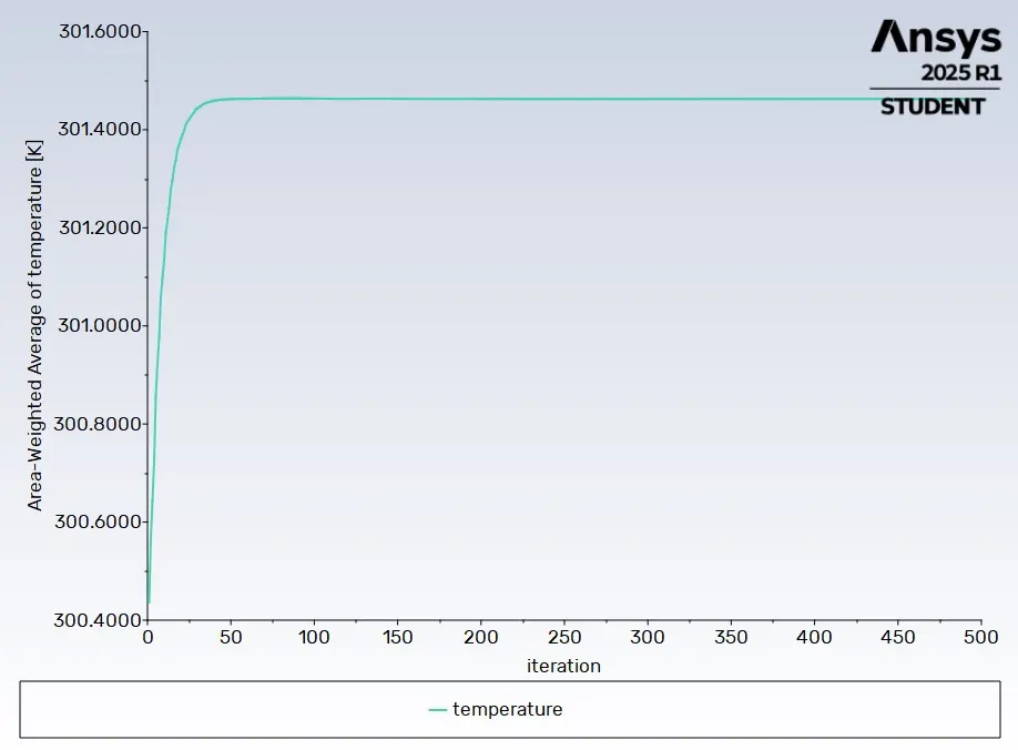
Heat transfer coefficient ( 3 m/sec ):

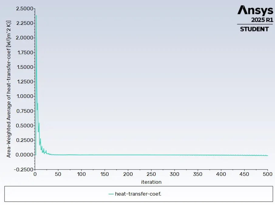
Case-3:

• Again we have go inside the boundaries then click on inlet .

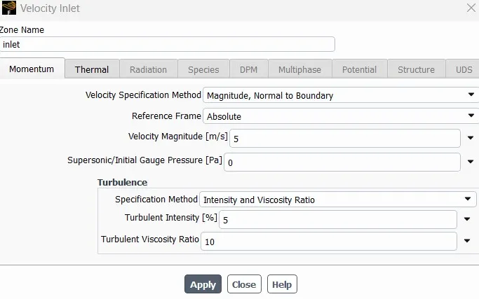
• We have to give the velocity magnitude is 5 m/sec .

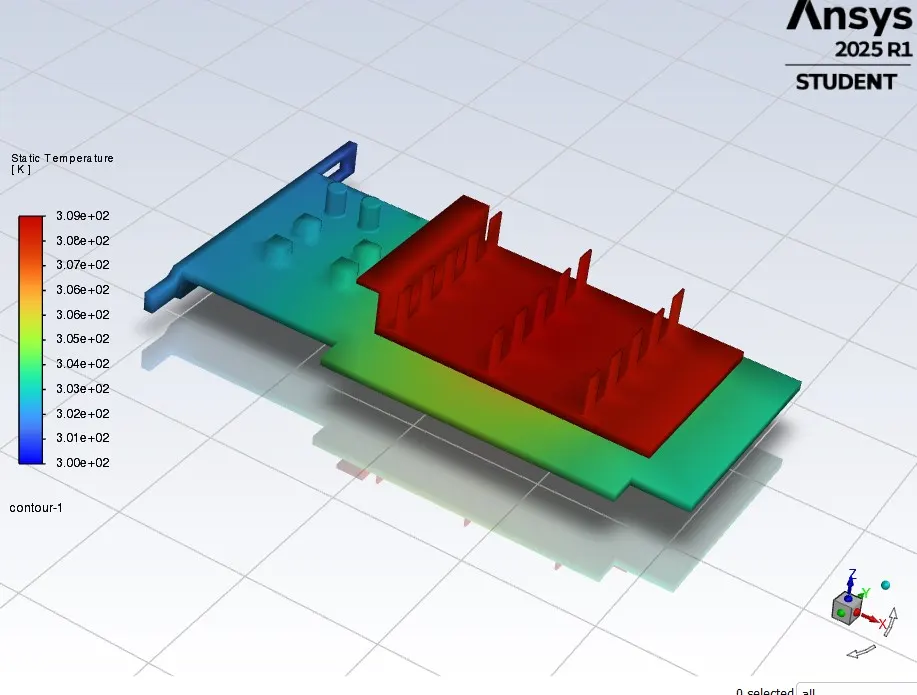
Temperature contour ( 5 m/sec ):

Residual Plot ( 5 m/sec ):

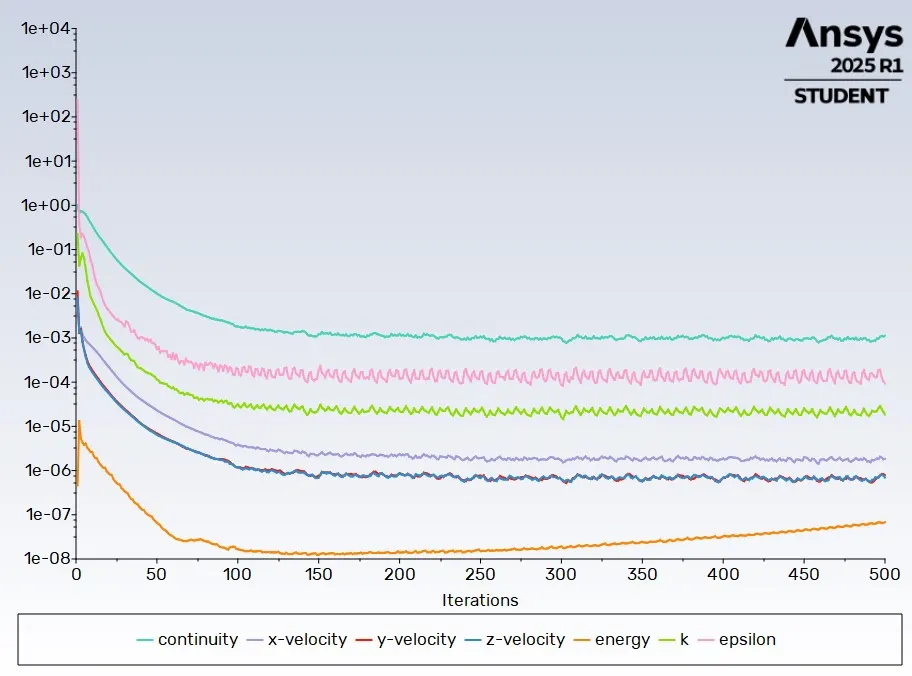
Temperature plot ( 5 m/sec ):

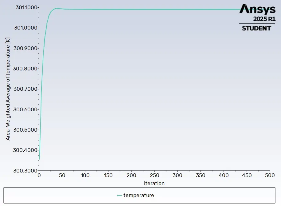
Heat transfer coefficient ( 5 m/sec ):

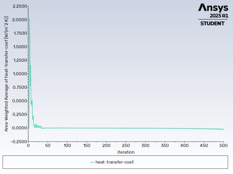
• From the above 3 cases we can compare the Heat Transfer coefficient of processer and Maximum Temperature.

• Inlet velocity (m/s)	Heat Transfer Coefficient	Temperature of processor(k)	Temperature of Fin(k)
  1	1.0729657	317.77657	317.51917
  3	2.9935517	311.44456	311.16152
  5	6.0901456	309.05809	308.76713

Refined mesh simulation :

• Again same procedure we have to follow whatever we did before in baseline mesh.

Case-1 :

Temperature contour ( 1 m/sec ):

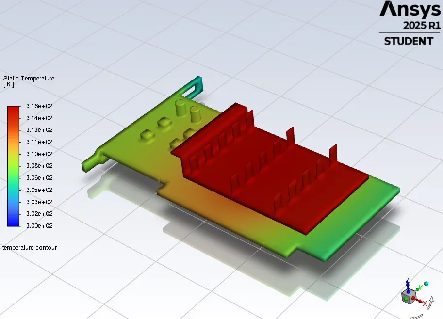
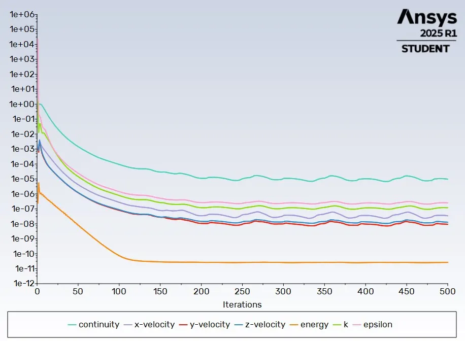
Residual Plot ( 1 m/sec ):

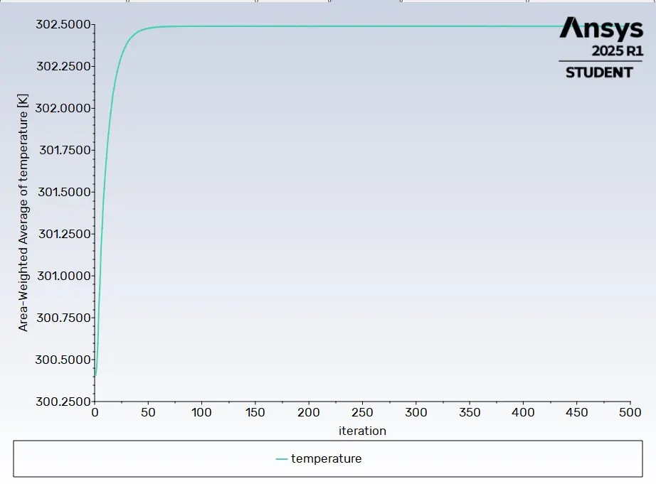
Temperature plot ( 1 m/sec ):

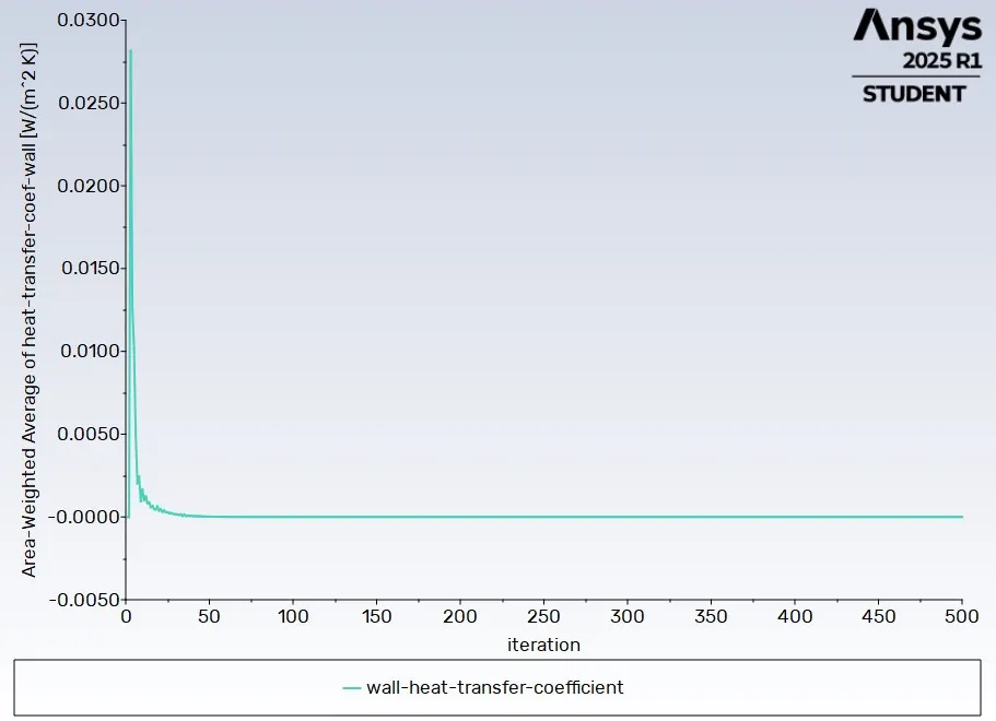
Heat transfer coefficient ( 1 m/sec ):

Case-2:

Temperature contour ( 3 m/sec ):

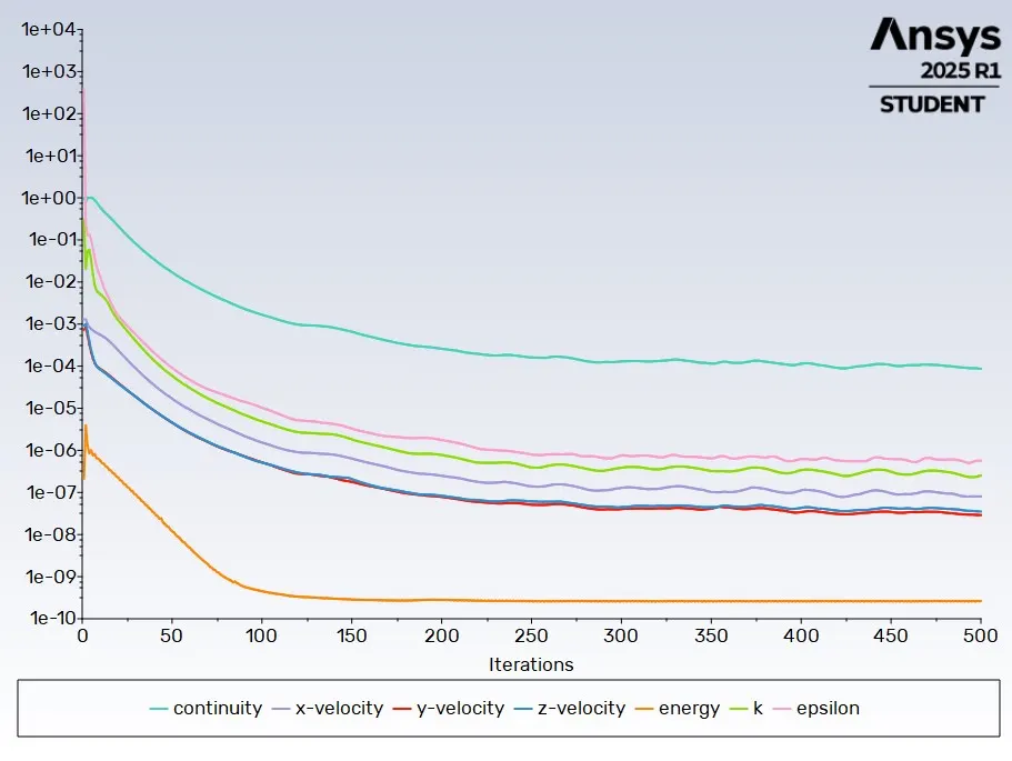
Residual Plot ( 3 m/sec ):

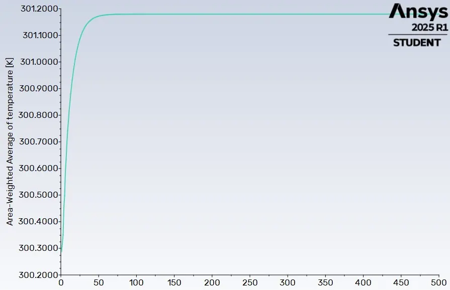
Temperature plot ( 3 m/sec ):

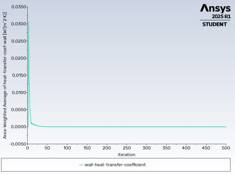
Heat transfer coefficient ( 3 m/sec ):

Case-3:

Temperature contour ( 5 m/sec ):

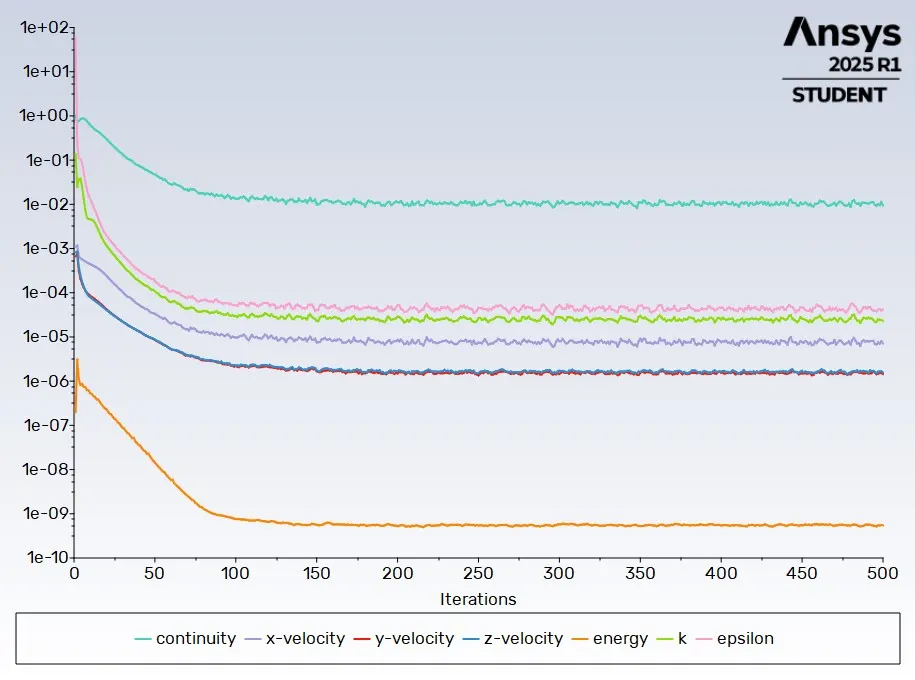
Residual Plot ( 5 m/sec ):

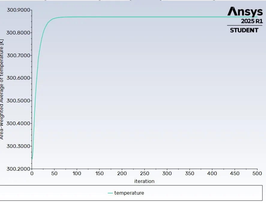
Temperature plot ( 5 m/sec ):

Heat transfer coefficient ( 5 m/sec ):

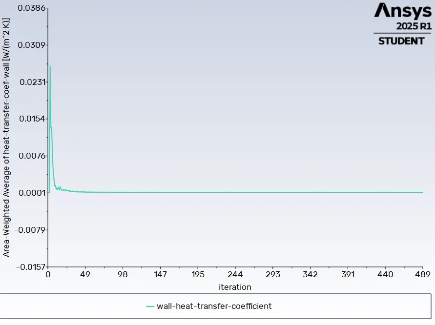
• From the above 3 cases we can compare the Heat Transfer coefficient of processer and Maximum Temperature.

• Inlet velocity (m/s)	Heat Transfer Coefficient	Temperature of processor(k)	Temperature of Fin(k)
  1	1.2498214	315.85347	315.64323
  3	2.528037	308.96496	308.73711
  5	6.5135319	307.13432	306.89942

Result setup :

Baseline mesh

• We have to click on Fin , Processer and Base and select the temperature then apply .
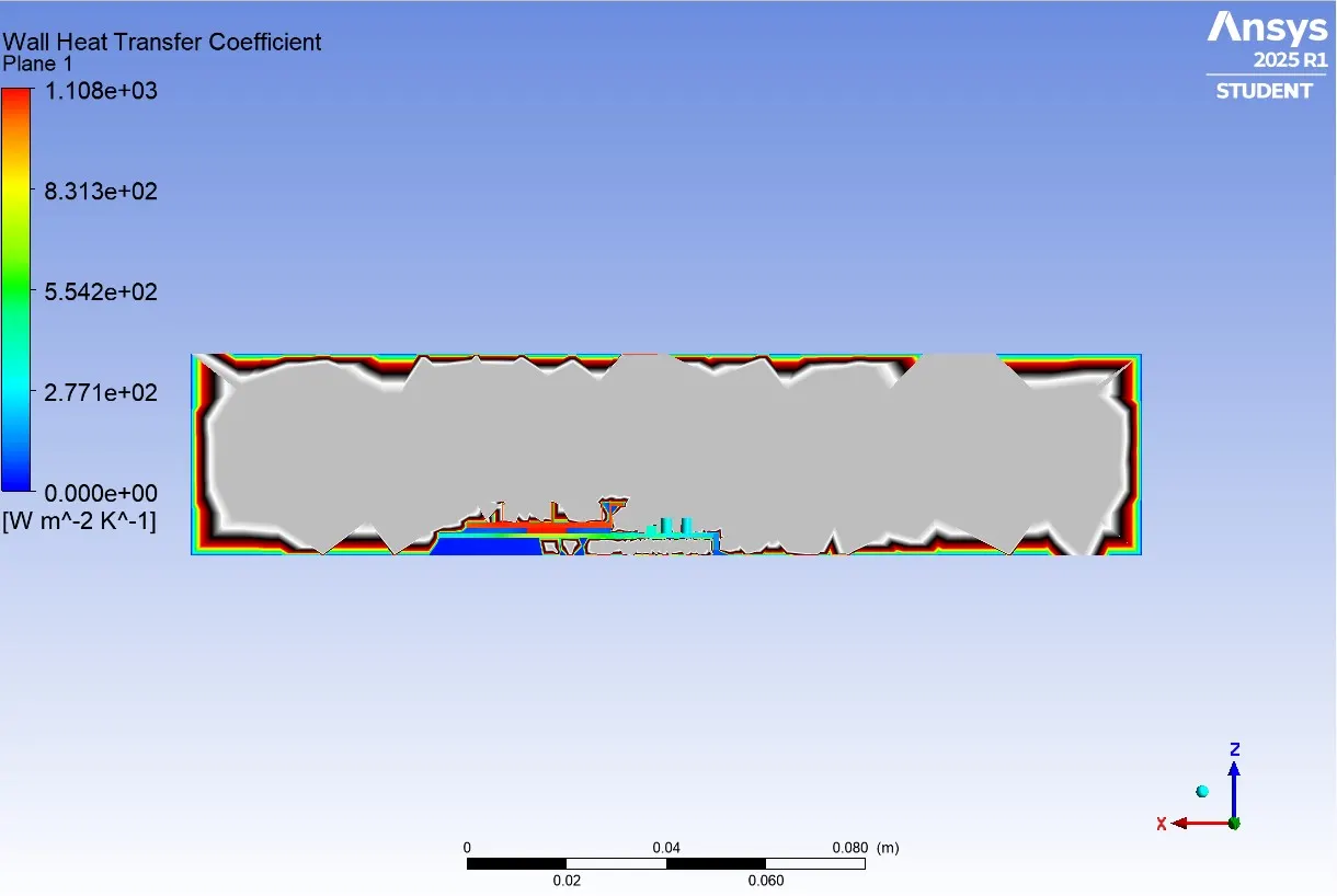
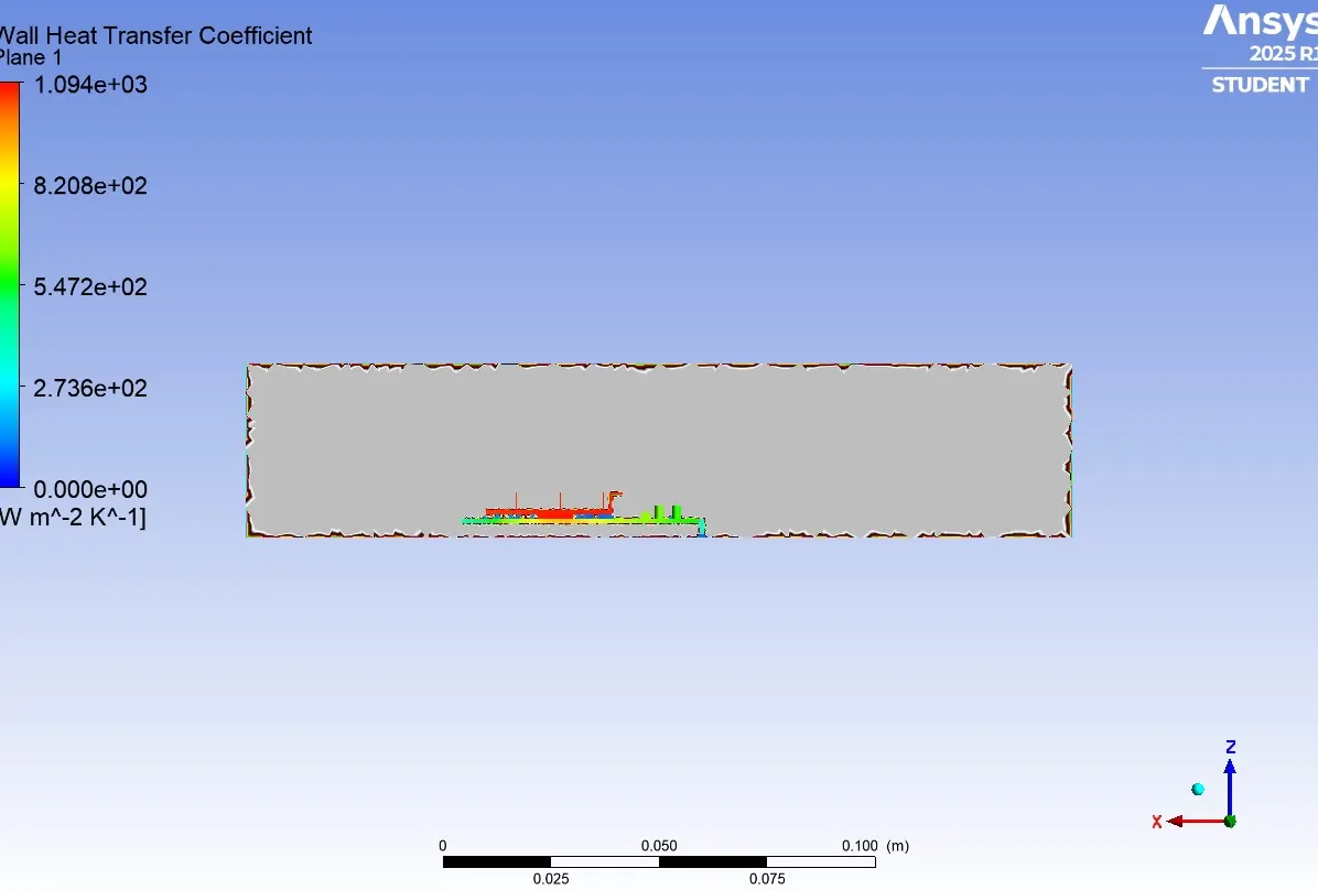
• We are going to create a plane inside result then we have to select the Wall heat transfer coefficient and apply.
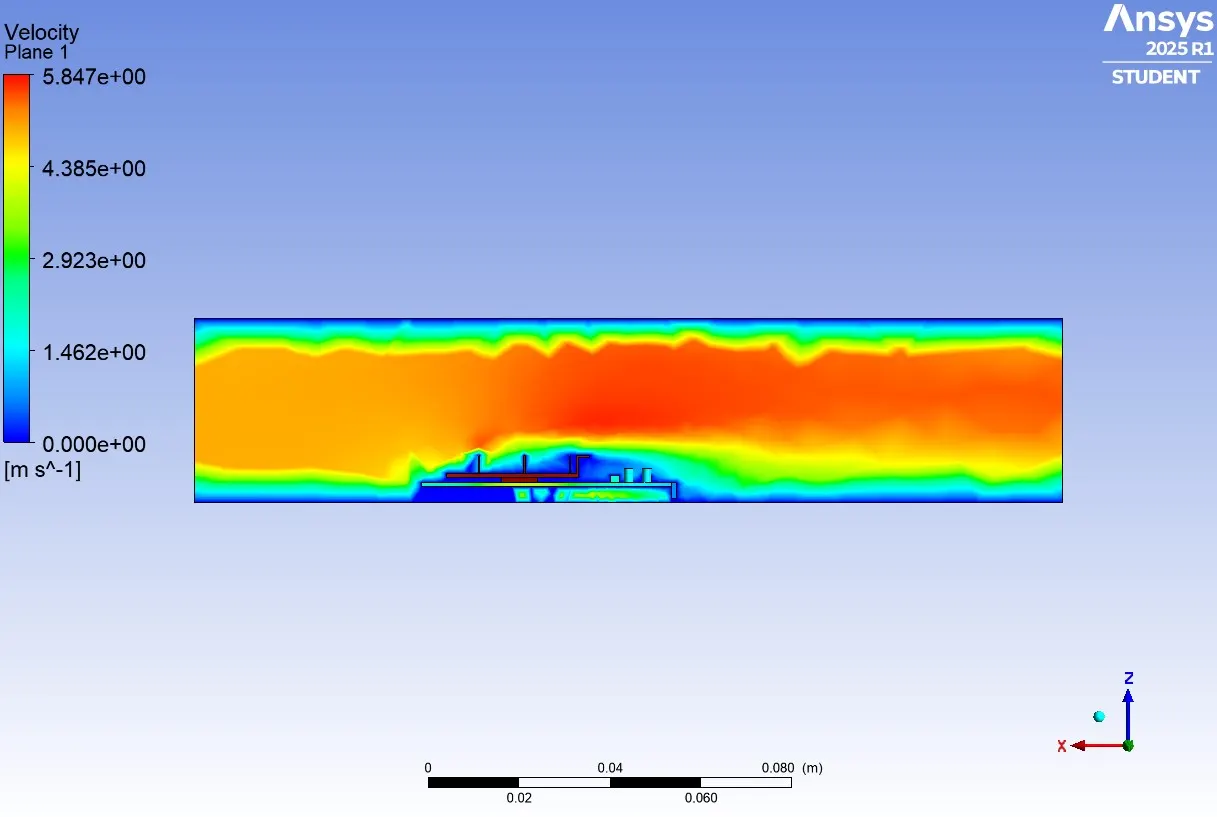
• Also we have to check the velocity inside the plane.

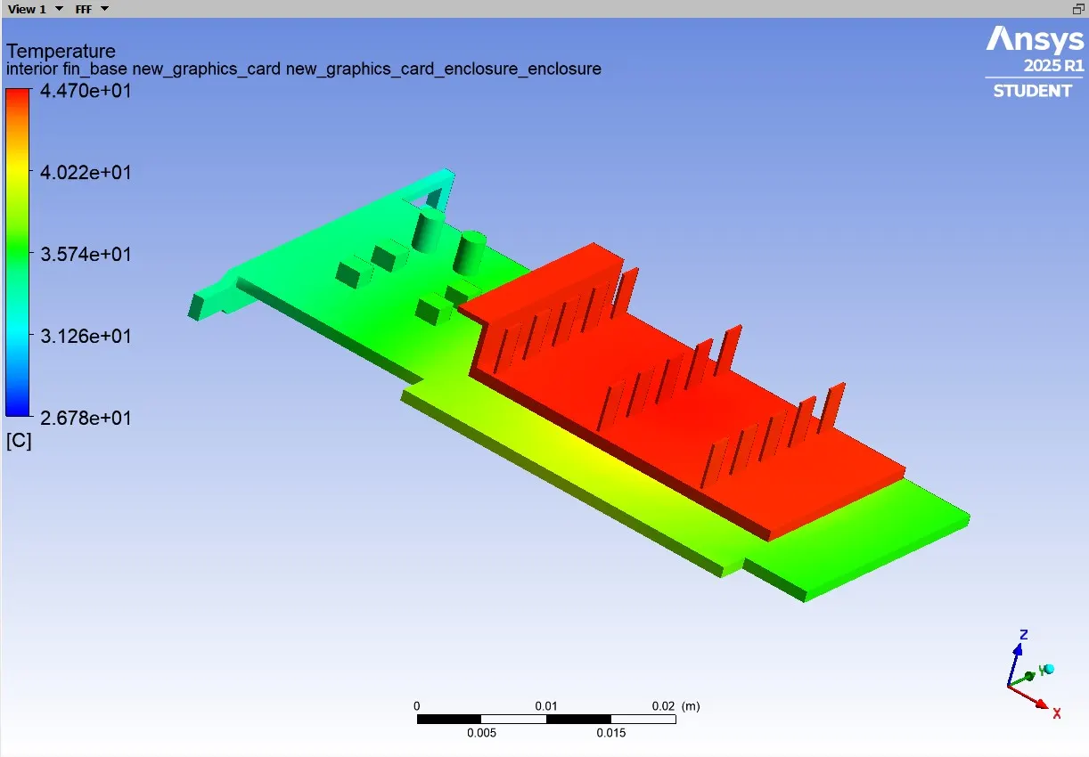
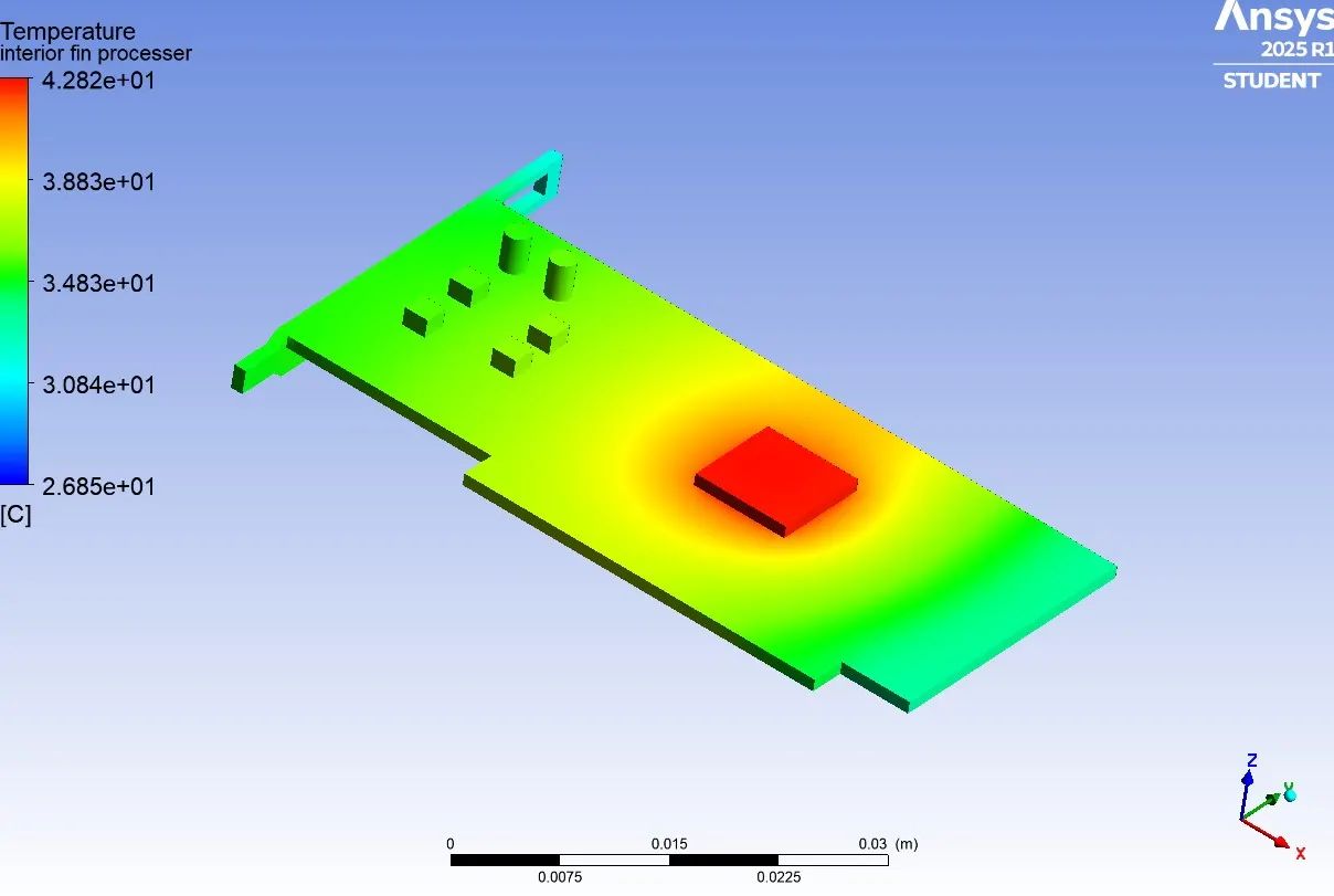
Hotspot around processer

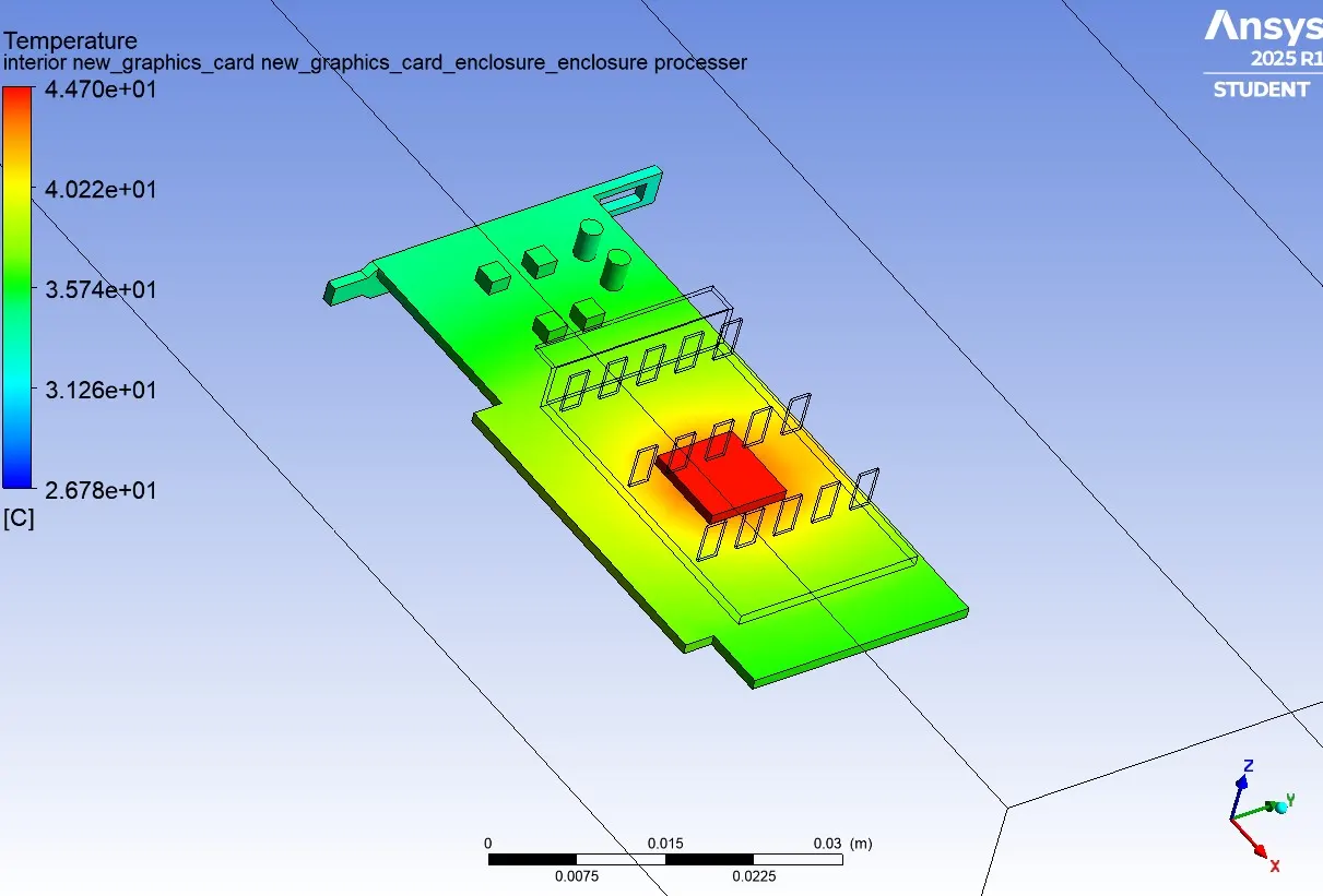
Wall Heat Transfer Coefficient

Velocity

Refined mesh :

Global Temperature

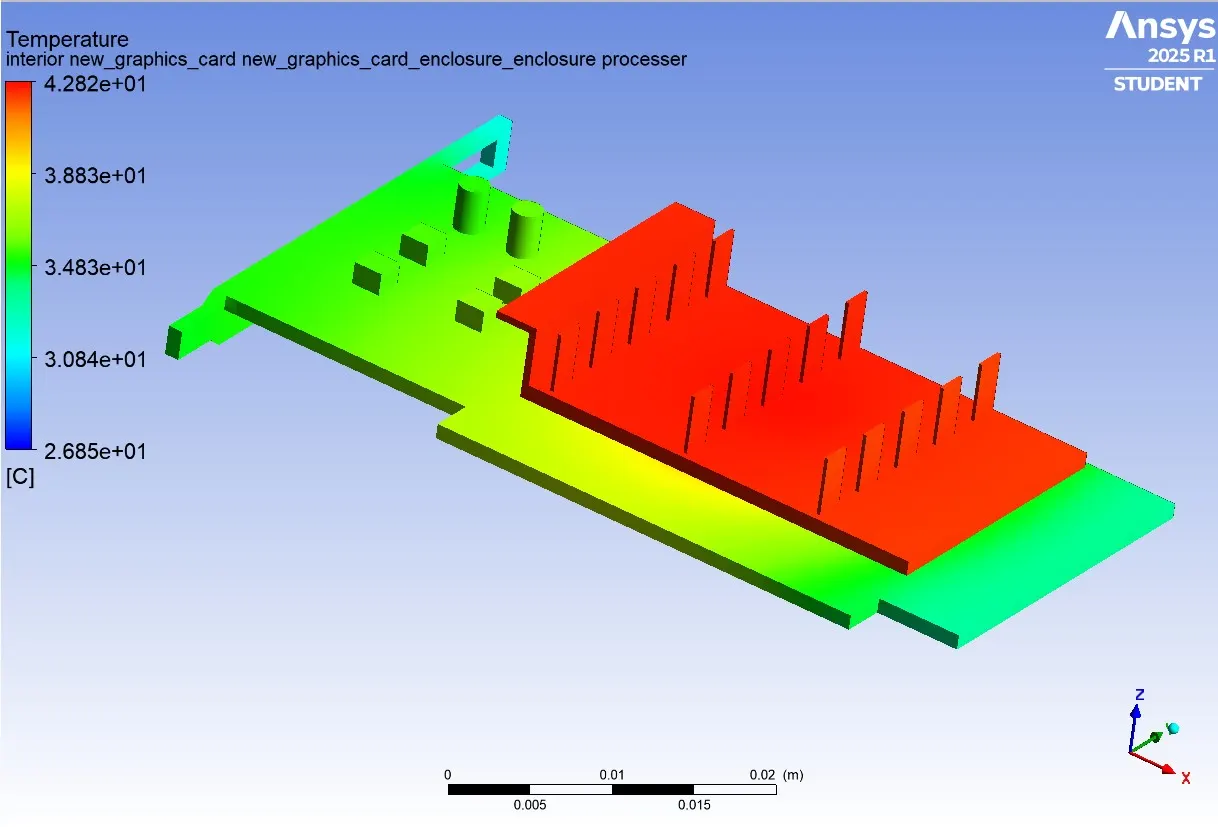
Hotspot around processer

Wall Heat Transfer Coefficient

Velocity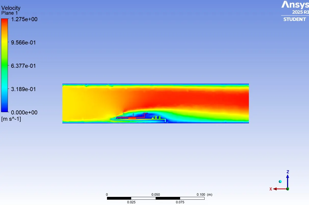

Conclusion:

• The thermal performance is seen to get improved increasing velocity of air and refining the mesh more.
• The maximum temperature of the processor is seen to decrease with the increase in velocity of air.
• The convergence criteria are satisfactorily achieved for baseline and refined mesh setup.
• We don't get that much good result in baseline mesh but In refined mesh we get good result as compare to baseline mesh.