Week 6 - CHT Analysis on a Graphics card

CHT analysis on Graphic card

Aim: To perform a steady-state conjugate heat transfer analysis on a model of a graphic card.

Introduction

Conjugate heat transfer analysis deals with heat transfer between fluids and solids. It basically helps in understanding temperature distributions between a fluid and solid at a particular zone. It has its applications in heat transfer in fins, electronic equipment such as PCBs, graphic cards, and various other heating and cooling systems.

Usually, to analyze a heat transfer environment, one needs to have an idea of the heat transfer coefficient. It is obtained by assuming a certain set of boundary conditions such as the heat being convicted in and out of the fluid and heat absorbed or rejected by the solid being considered. This is not easy as the parameters change from time to time. So, these assumptions prove to be erroneous and complex. So, to analyze the given condition, we consider the conjugating boundary condition at the solid-liquid interface. This is a coupled analysis that is used in situations that consist of situations involving heat transfer governed by multiple governing equations. We solve the corresponding governing equations for a corresponding sub-domain and conjugate them at a solid and liquid interface.

Theory:

Heat transfer in solids

Heat transfer in solids is defined by Fourier's law of heat conduction. It means that the heat transfer through a solid is directly proportional to the temperature gradient. If the heat transfer is transient, then the Fourier's law is given by:

Q=−KAdT/dx

Q - Heat transfer happening in the material

K - Thermal conductivity of the material

A - cross-sectional area of the material

dT/dx - Temperature gradient in the material

Heat transfer in liquids and gases

Heat transfer in liquids and gases takes by means of convection due to the differences in density. It is given by the following equation.

Q=hA△T

Q - Heat transfer happening in the material

h - Convective heat transfer of the material

A - cross-sectional area of the material

△T - Temperature difference in the process

Conjugate heat transfer analysis is the analysis where we consider both the combination of conduction in solids and convection in gases.

Setting up the problem :

Geometry

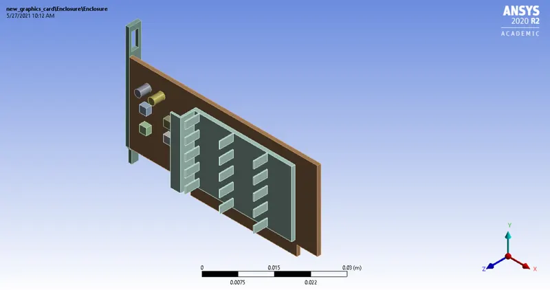
Fig 1: Geometry of a graphic card model

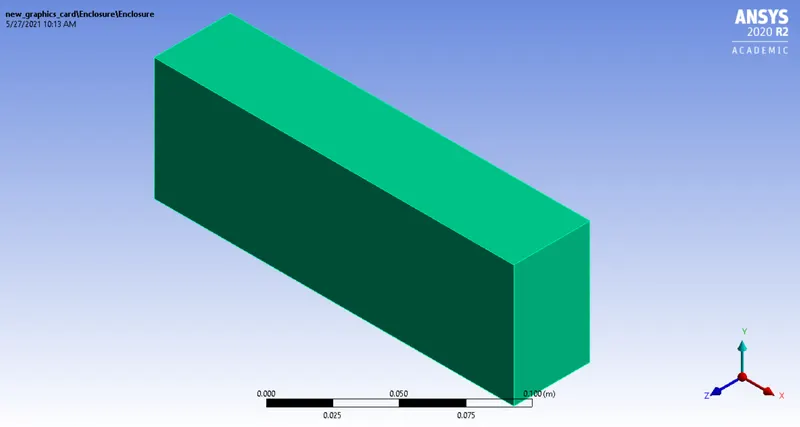
Fig 2: Enclosure surrounding the graphic card

Meshing

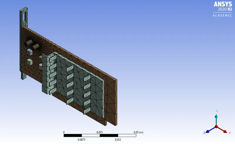
Fig 3: Baseline mesh of the graphic card

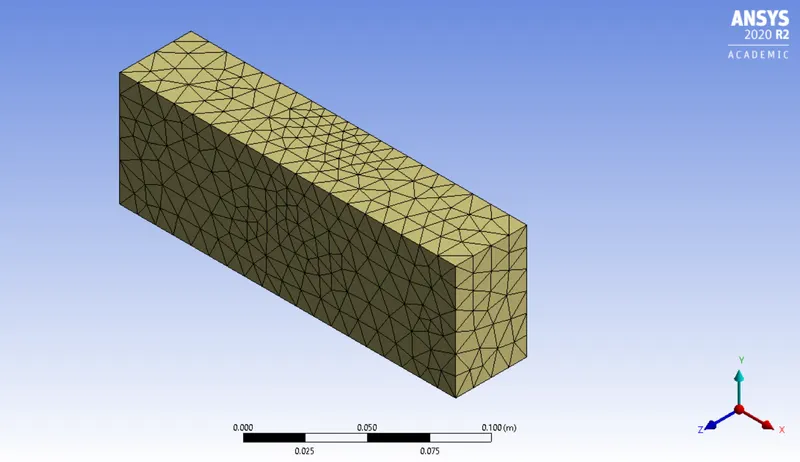
Fig 4: Baseline mesh of the enclosure

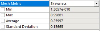
Fig 5: Mesh metric (skewness) for baseline mesh

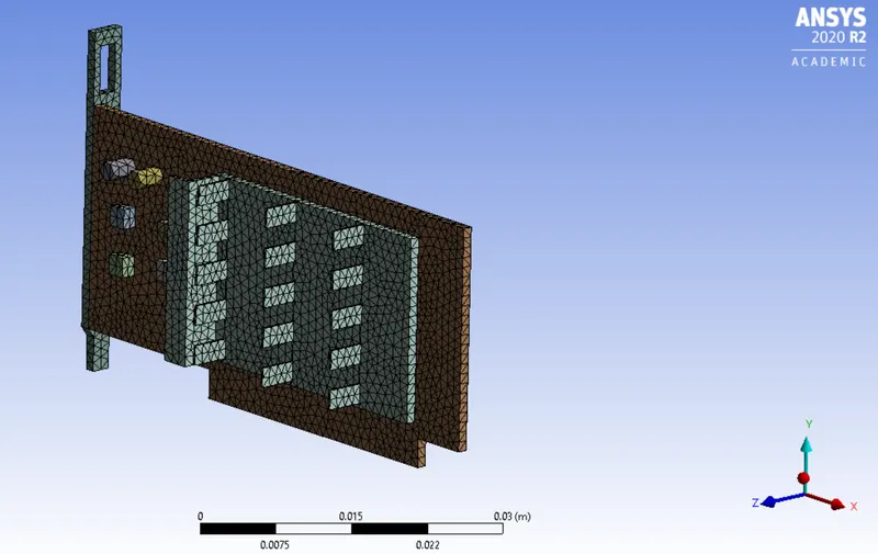
Fig 6: Refined mesh for the graphic card

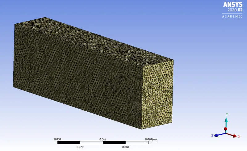
Fig 7: Refined mesh for the enclosure

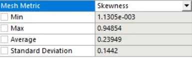
Fig 8: Mesh metric (skewness) for refined mesh

• For baseline mesh, default mesh with 84,244 elements and 15776 nodes.
• For a refined mesh, different body sizings at appropriate locations have been applied which resulted in 297976 elements and 54029 nodes.

  • Location	Element size (m)
    Enclosure	2.5e-3
    Fins	1.0e-3
    Processor	1.0e-3
    Base	1.0e-3

Table 1: Mesh details

• Skewness has been considered as a mesh metric. In the baseline mesh, skewness is as low as 1.305e-10. Whereas it got improved to 1.13e-3 with refinement.
  
  • The reason for choosing this refinement is that on further refinement, there were certain errors where mesh being not recorded or exceeding the eligible element count. I personally feel that the mesh could be furthermore refined.

Location	Material
Enclosure	Air
Fins	Aluminum
Base	Copper
Processor	Silicon

Table 2: Material properties

Boundary conditions

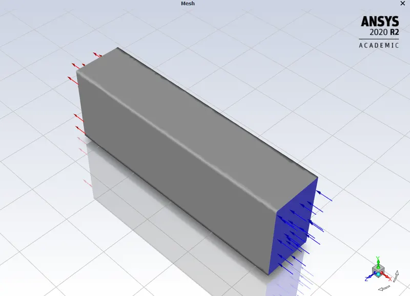
Fig 9: Boundary conditions applied

Following are the boundary conditions applied for this simulation

Location	Boundary conditions for run 1	Boundary condition for run 2	Boundary condition for run 3
Inlet	1 m/sec	3 m/sec	5 m/sec
Outlet	Atm. pressure	Atm. pressure	Atm. pressure
Processor	5e5 W/m^2	5e5 W/m^2	5e5 W/m^2

Table 3: Boundary conditions

The heat flux emanating from the processor has been considered as 5e5 W/m^2. This is done by assuming the wattage of the processor to be 40 W and the surface area of the flux is 80e-6 m^2.

With the above boundary conditions 6 runs were done (each run with 2 mesh sizes).

Following are the settings considered for solving this problem:

Energy equation	On
Type of analysis	Steady-state
Turbulent theory considered	k-e
Schemed used	Pressure-velocity coupled
Residuals monitored	1e-6 for every equation, 1e-15 for energy

Note: The simulation was initialized using standard initialization computed from inlet and also temperature is set at 300 K.

Table 4: Settings considered for solving

Results

Temperature distributions for various locations of the graphic card and wall heat transfer coefficient distributions have been attached here.

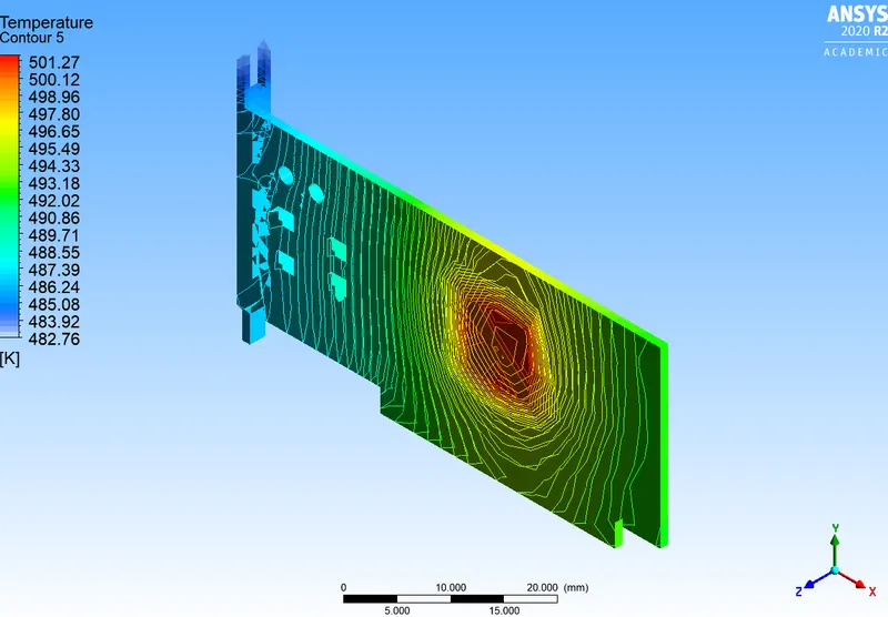
Fig 10: Temperature distribution for the base when V= 1m/sec for baseline mesh

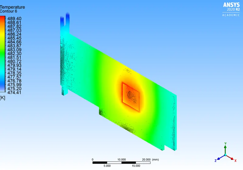
Fig 11: Temperature distribution for the base when V= 1m/sec for refined mesh

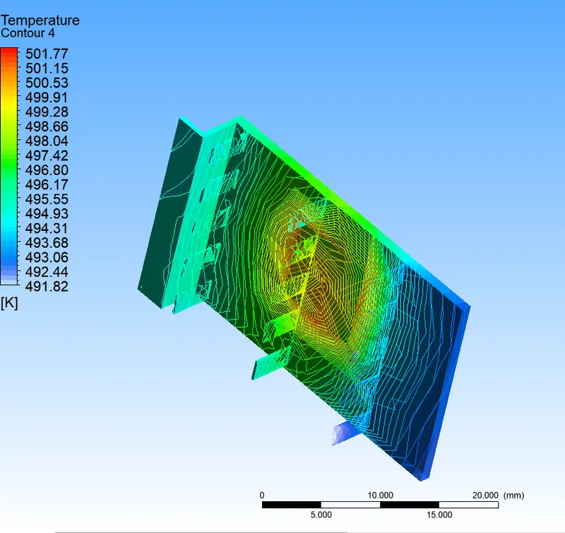
Fig 12: Temperature distribution for fins when V= 1m/sec for baseline mesh

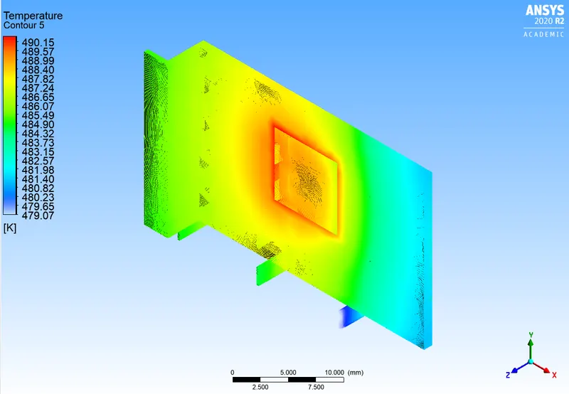
Fig 13: Temperature distribution for fins when V= 1m/sec for refined mesh

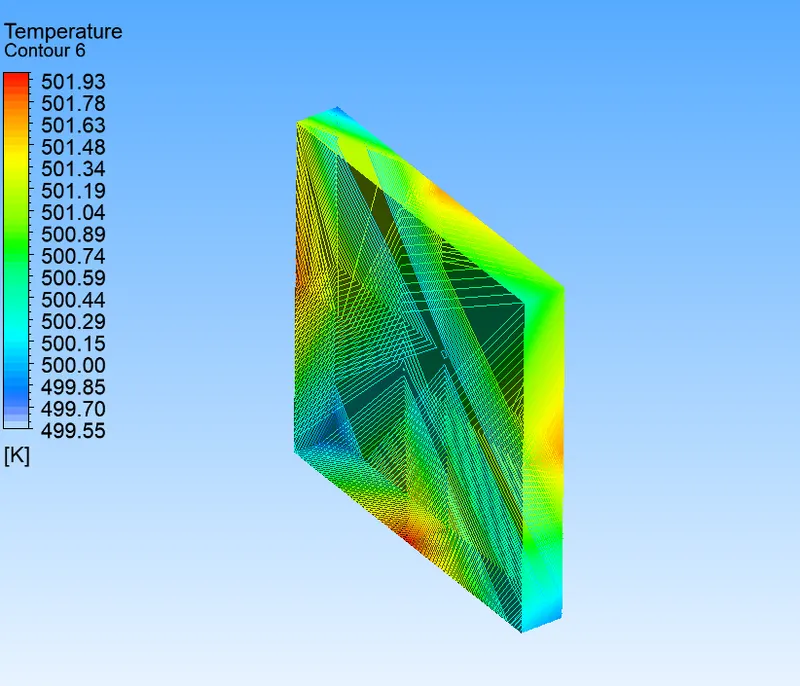
Fig 14: Temperature distribution for the processor when V= 1m/sec for baseline mesh

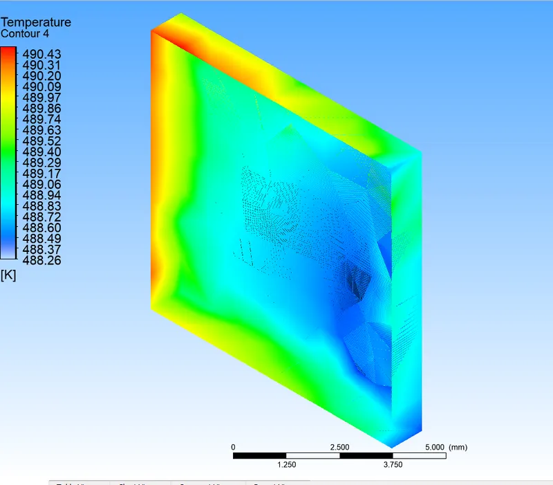
Fig 15: Temperature distribution for processor when V= 1m/sec for refined mesh

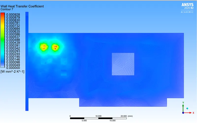
Fig 16: Wall heat transfer coefficient when V= 1m/sec for baseline mesh

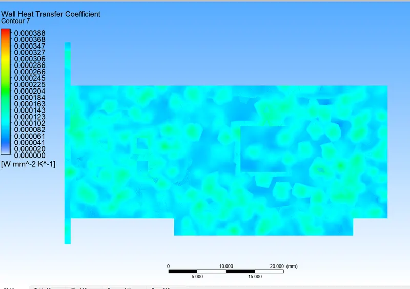
Fig 17: Wall heat transfer coefficient when V= 1m/sec for refined mesh

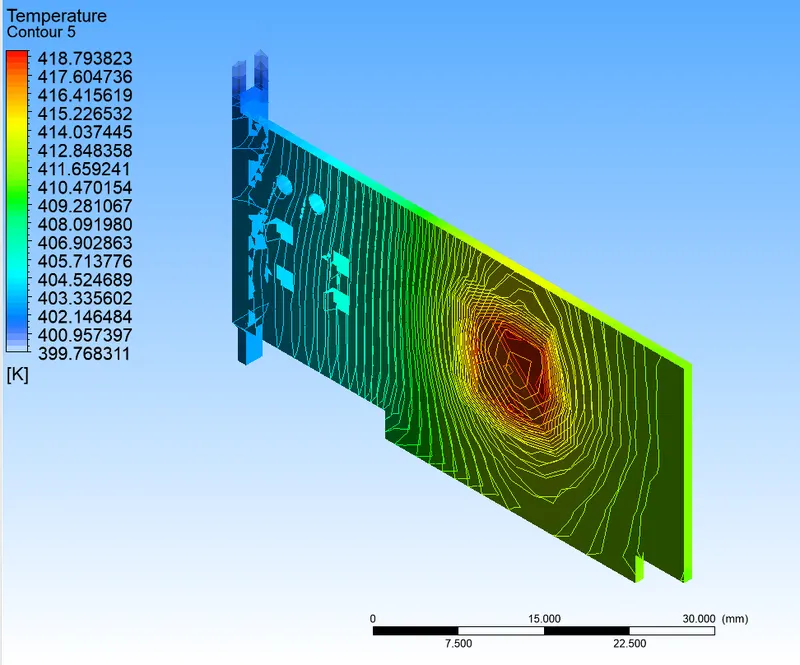
Fig 18: Temperature distribution for the base when V= 3 m/sec for baseline mesh

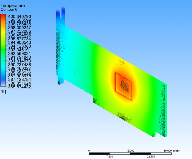
Fig 19: Temperature distribution for the base when V= 3 m/sec for refined mesh

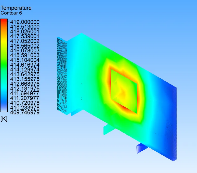
Fig 20: Temperature distribution for fins when V= 3 m/sec for baseline mesh

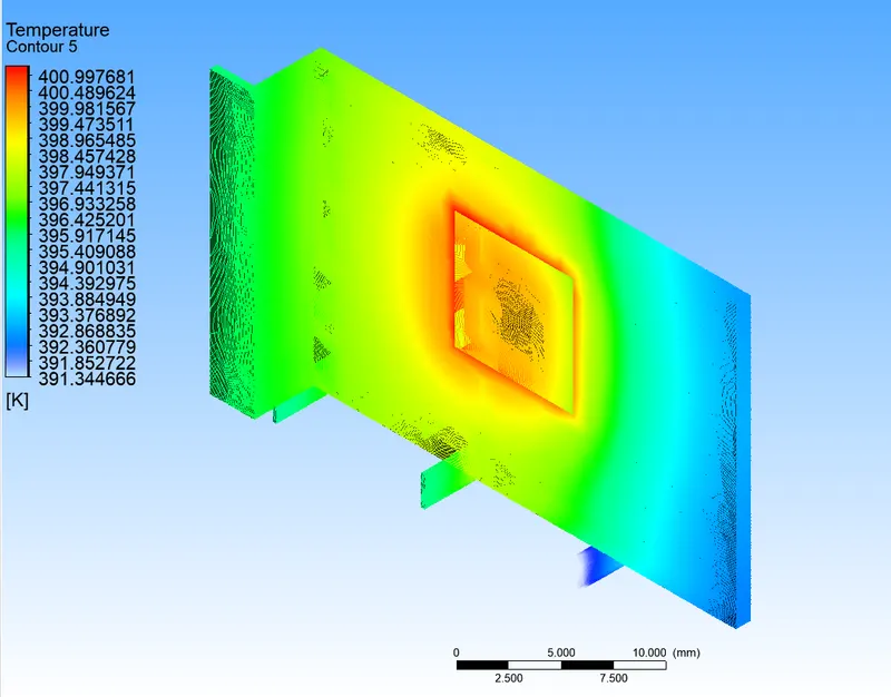
Fig 21: Temperature distribution for fins when V= 3 m/sec for refined mesh

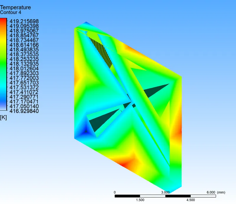
Fig 22: Temperature distribution for the processor when V= 3 m/sec for baseline mesh

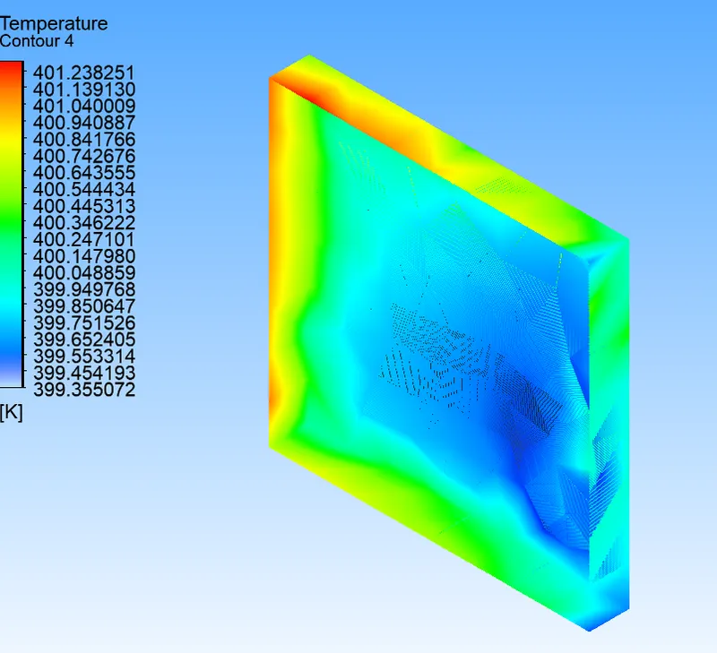
Fig 23: Temperature distribution for the processor when V= 3 m/sec for refined mesh

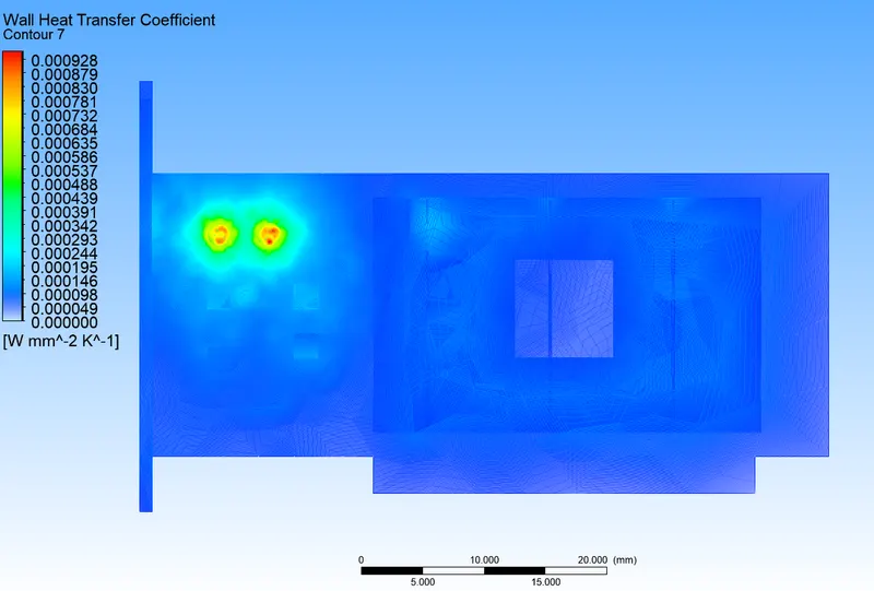
Fig 24: Wall heat transfer coefficient when V= 3 m/sec for baseline mesh

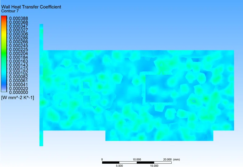
Fig 25: Wall heat transfer coefficient when V= 3 m/sec for refined mesh

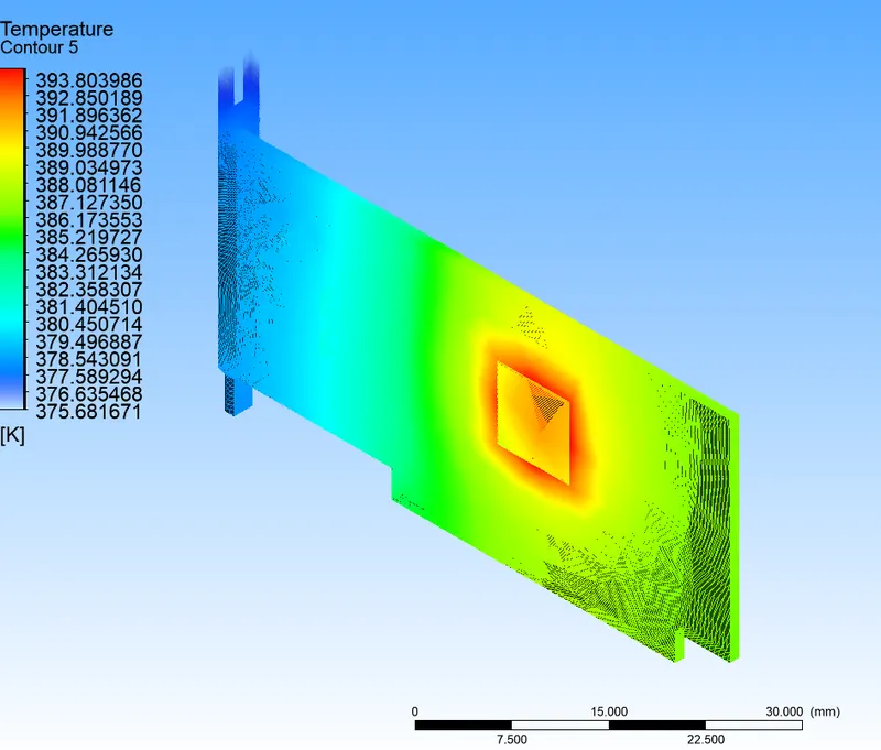
Fig 26: Temperature distribution for the base when V= 5 m/sec for baseline mesh

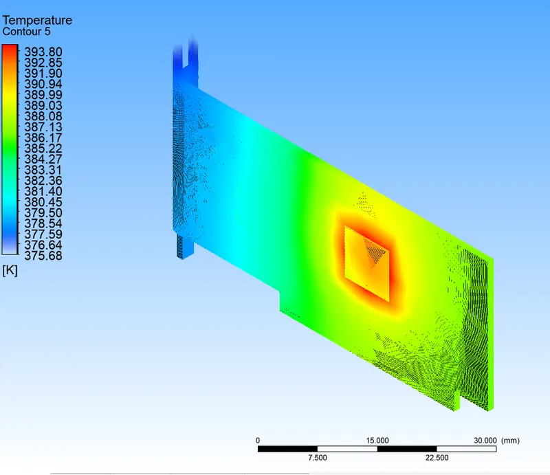
Fig 27: Temperature distribution for the base when V= 5 m/sec for refined mesh

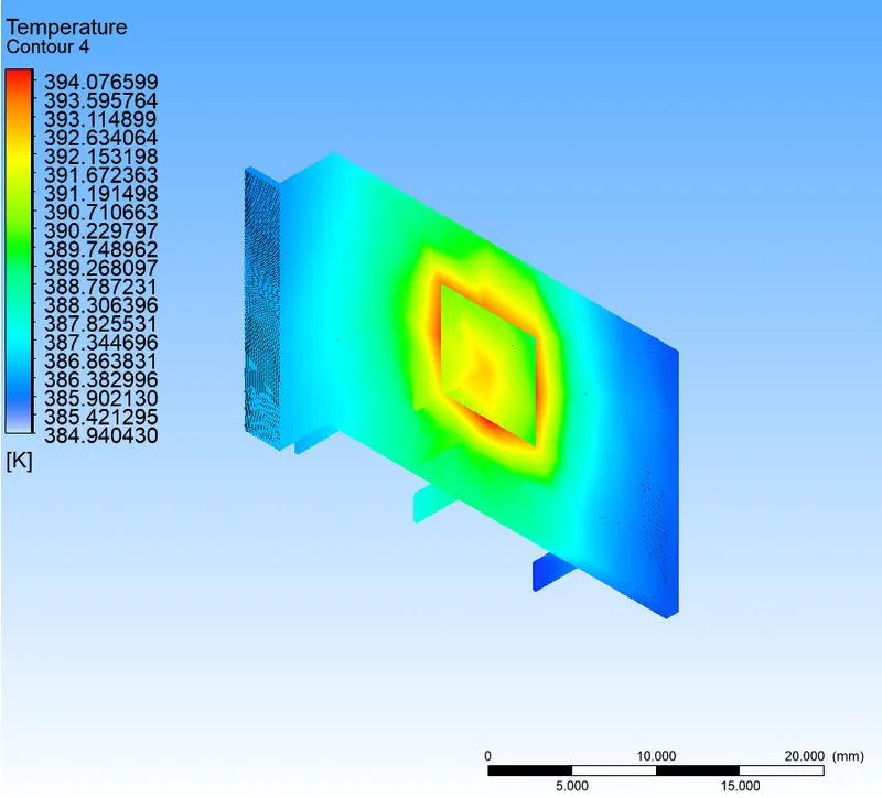
Fig 28: Temperature distribution for fins when V= 5 m/sec for baseline mesh

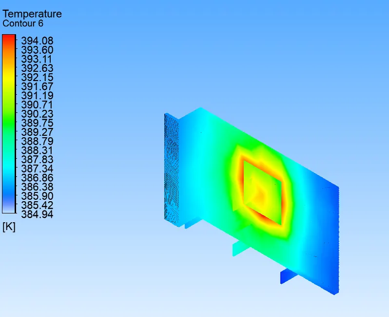
Fig 29: Temperature distribution for fins when V= 5 m/sec for refined mesh

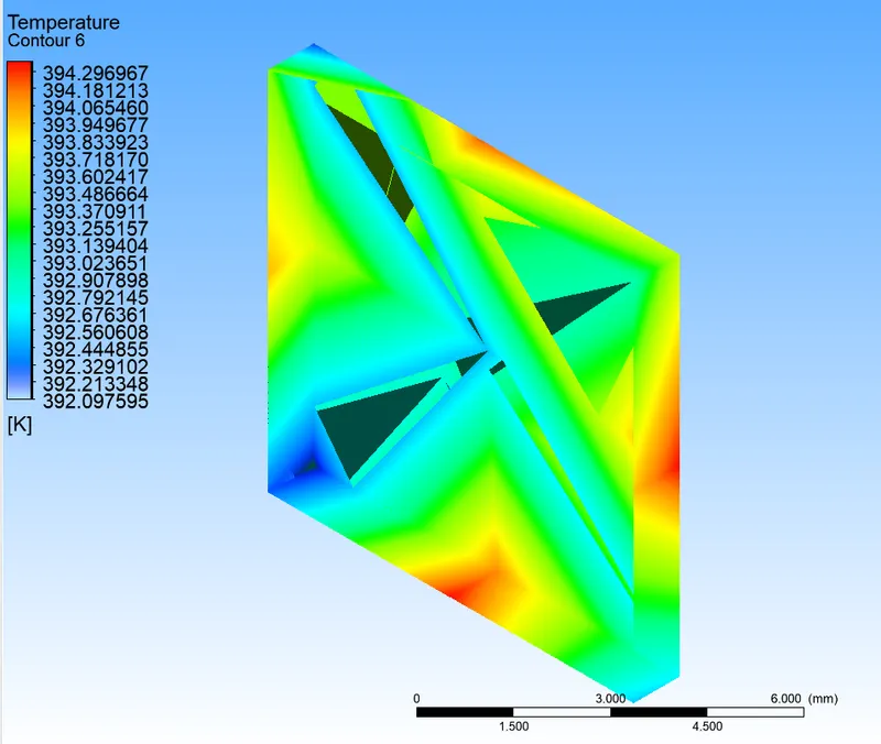
Fig 30: Temperature distribution for the processor when V= 5 m/sec for baseline mesh

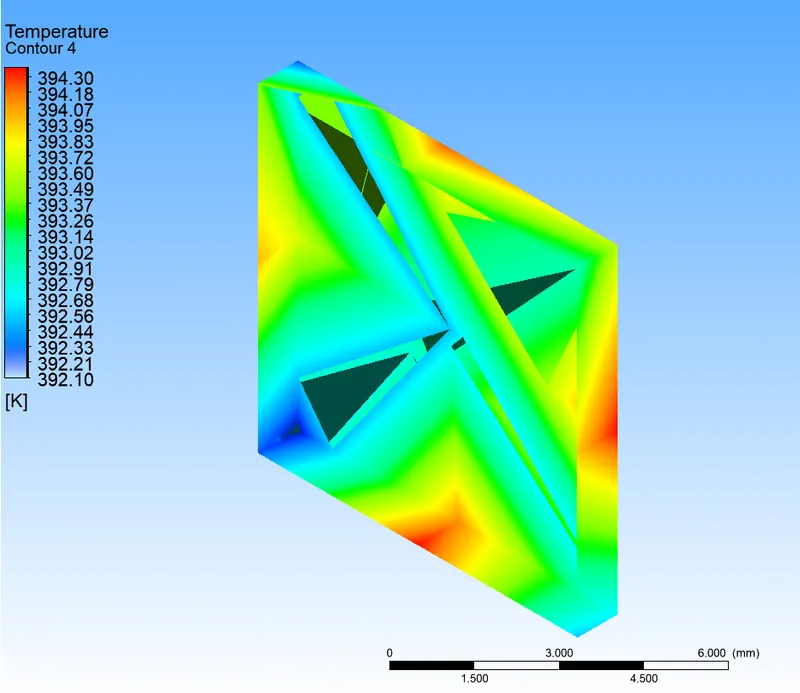
Fig 31: Temperature distribution for the processor when V= 5 m/sec for refined mesh

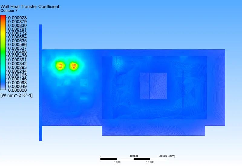
Fig 32: Wall heat transfer coefficient when V= 5 m/sec for baseline mesh

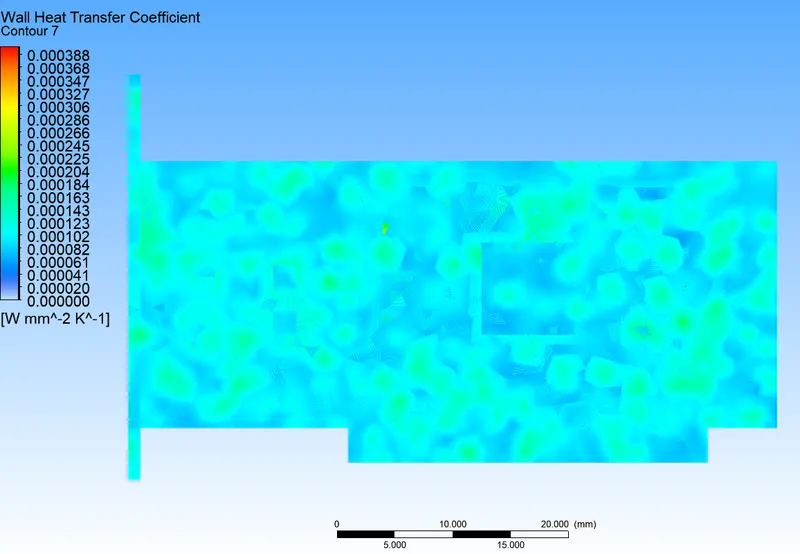
Fig 33: Wall heat transfer coefficient when V= 5 m/sec for refined mesh

Inferences

Property	Baseline mesh for 1 m/sec	Refined mesh for 1 m/sec	Baseline mesh for 3 m/sec	Refined mesh for 3 m/sec	Baseline mesh for 5 m/sec	Refined mesh for 5 m/sec
Tmin(Base)	482.76 K	474.41 K	399.77 K	385.58 K	375.68 K	366.00 K
Tmax(Base)	501.27 K	489.40 K	418.80 K	400.35 K	393.80 K	380.26 K
Tmin(Fins)	491.82 K	479.07 K	409.75 K	391.35 K	384.94 K	371.77 K
Tmax(Fins)	501.77 K	490.15 K	419.00 K	401.00 K	394.07 K	380.81 K
Tmin(Processor)	499.55 K	488.26 K	416.93 K	399.36 K	392.09 K	379.36 K
Tmax(Processor)	501.93 K	490.43 K	419.22 K	401.24 K	394.30 K	381.06 K
Wall heat transfer coefficient (max)	0.000928 W mm^-2 K^-1	0.000388 W mm^-2 K^-1	0.000928 W mm^-2 K^-1	0.000388 W mm^-2 K^-1	0.000928 W mm^-2 K^-1	0.000388 W mm^-2 K^-1

Table 5: Temperature distribution across various locations

From the above table following inferences can be made:

• There is a significant change in temperature distribution at every location with the refinement of the mesh.
• Velocity plays an important role here. One can observe that with the increase in velocity of air, the increase in the temperature due to the processor's heat flux is restricted to a lower value due to the heat lost in convection.
• The highest possible rise in temperature can be seen in the processor as the heat flux emanates from it.
• There is not so much change in wall heat transfer coefficient with the change in velocity.

Gaps:

• One more iteration should be considered for this simulation.
• One major shortcoming in this challenge might be the selection of the processor's material and availability of material properties.
• In this case, silicon has been considered as the material where as in reality silicon along with other materials are used.