Exhaust Port Challenge

EXHAUST PORT CHALLENGE

AIM AND OBJECTIVES

1. To give a brief description of why and where CHT analysis is used.

2. To maintain the y+ value according to the turbulence model and justify the results

3. To calculate the wall/surface heat transfer coefficient on the internal solid surface and to show the velocity and temperature contours in appropriate areas.

4. To verify if the CHT predictions of the simulation are right and to analyze what factors does the accuracy of the prediction depends on.

INTRODUCTION

CHT (Conjugate Heat Transfer) analysis :

This type of heat transfer is considered to be a combination of heat transfer in solids and heat transfer in liquids. This kind of heat transfer is usually observed in many real-life situations. They range from heat transfer in a circuit board to heat transfer in a space vehicle or a nuclear plant.

Usually, in order to analyze a heat transfer environment, one needs to have an idea of the heat transfer coefficient and it is obtained by assuming a certain set of boundary conditions such as the heat being convicted in and out of the fluid and heat absorbed or rejected from the solid being considered. This is not easy as the parameters change from time to time. So, these assumptions prove to be erroneous and complex. So, in order to analyze the given condition, we consider the conjugating boundary condition at the solid-liquid interface. This is a coupled analysis that is used in situations that consist of situations involving heat transfer governed by multiple governing equations. We solve the corresponding governing equations for a corresponding sub-domain and conjugate them at the interface of solid and liquid.

The best situation where CHT analysis could be applied is the case where a solid conducting heat from inside is in the environment of an external fluid.

Applications: Continous casting, extrusion, rolling and forming, and other manufacturing processes.

Theory:

Heat transfer in solids

Heat transfer in solids is defined by Fourier's law of heat conduction. It means that the heat transfer through a solid is directly proportional to the temperature gradient. If the heat transfer is transient, then the Fourier's law is given by:

Q=−KAdT/dx

Q - Heat transfer happening in the material

K - Thermal conductivity of the material

A - cross-sectional area of the material

dT/dx - Temperature gradient in the material

Heat transfer in liquids and gases

Heat transfer in liquids and gases takes by means of convection due to the differences in density. It is given by the following equation.

Q=hA△T

Q - Heat transfer happening in the material

h - Convective heat transfer of the material

A - cross-sectional area of the material

△T - Temperature difference in the process

Conjugate heat transfer analysis is the analysis where we consider both the combination of conduction in solids and convection in gases.

Wall y+: It is the non-dimensional distance from the wall to the first mesh node. Too large y+ values will make the first mesh node to be outside the boundary layer and this results in incorrect calculation of the flow properties. For k-e turbulence theory typically wall y+ is considered between 30 and 300.

Setting up the problem :

Geometry

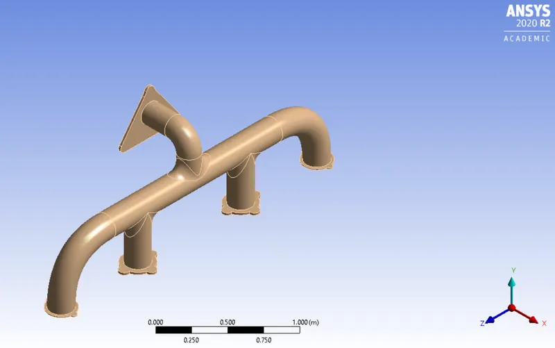
Fig 1: Geometry of the model considered

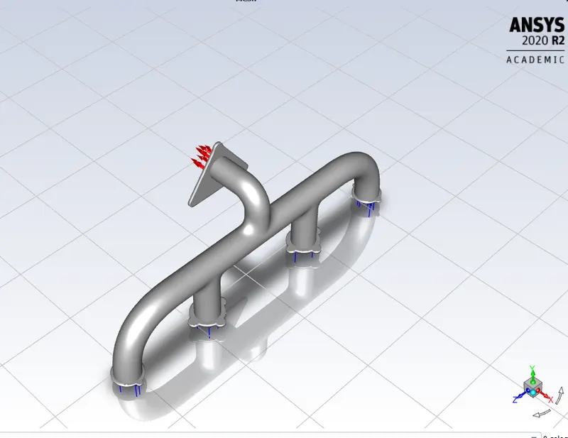
Fig 2: Boundary conditions

In this simulation following boundary conditions are considered.

Inlet conditions:

There are 4 inlets in total.

Velocity = 5 m/sec

Temp = 700 K

Outlet conditions :

△Q=0 (Adiabatic condition)

Outer wall convection :

h = 20 W/m^2 K

Temp = 300 K

Simulations:

A total of three simulations have been run. They are,

1) Overall mesh size for element being 0.15 m.

2) Overall mesh size for the element being 0.15 m and an inflation layer over the walls being 2.5 mm thick.

3) Overall mesh size for the element being 0.15 m and a body sizing of 0.01 m on solid volume with an inflation layer of 5 mm thickness.

The fluid under consideration is air and the solid chosen is Aluminum by default.

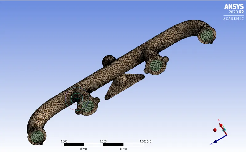
Fig 3: Mesh for run 1

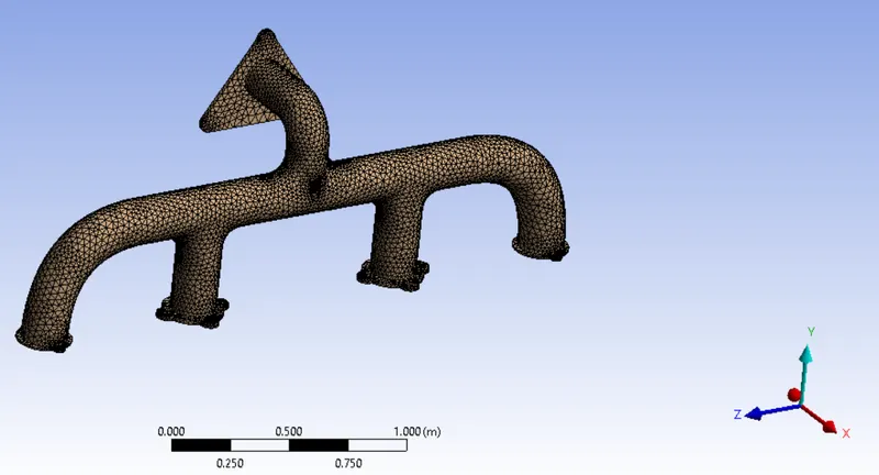
Fig 4: Mesh for run 2

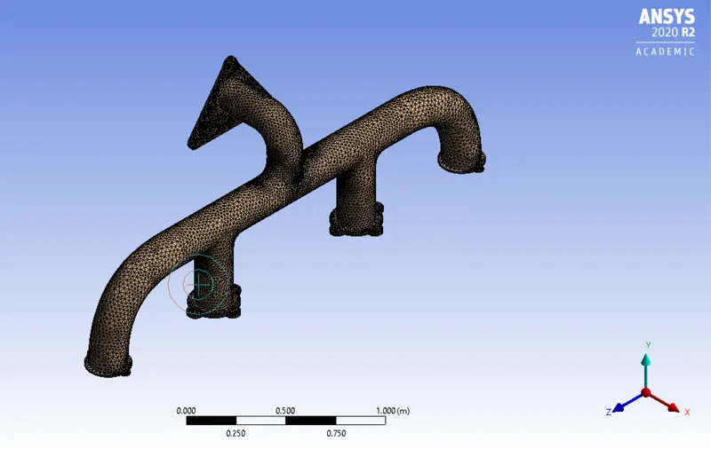
Fig 5: Mesh for run 3

This was done to check the effect of inflation on the results. As we know the inflation layer captures the boundary layer phenomenon. Following are the results that have been obtained from these runs.

Results:

1) For run 1

No of elements = 137492

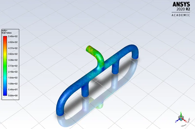
Fig 6. y+ values for run 1

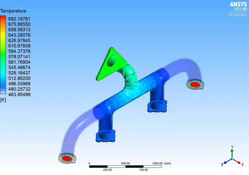
Fig 7. Temperature contours for run 1

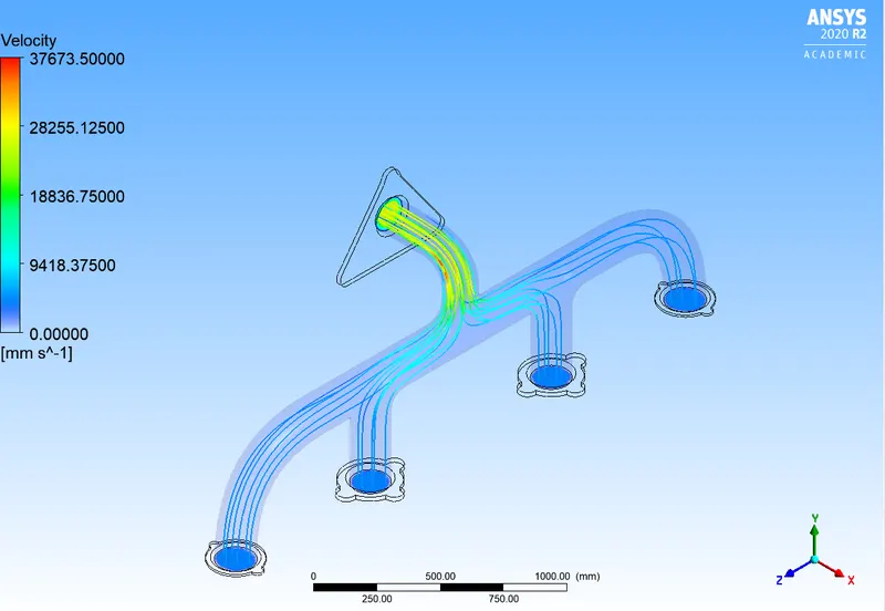
Fig 8. Velocity streamlines for run 1

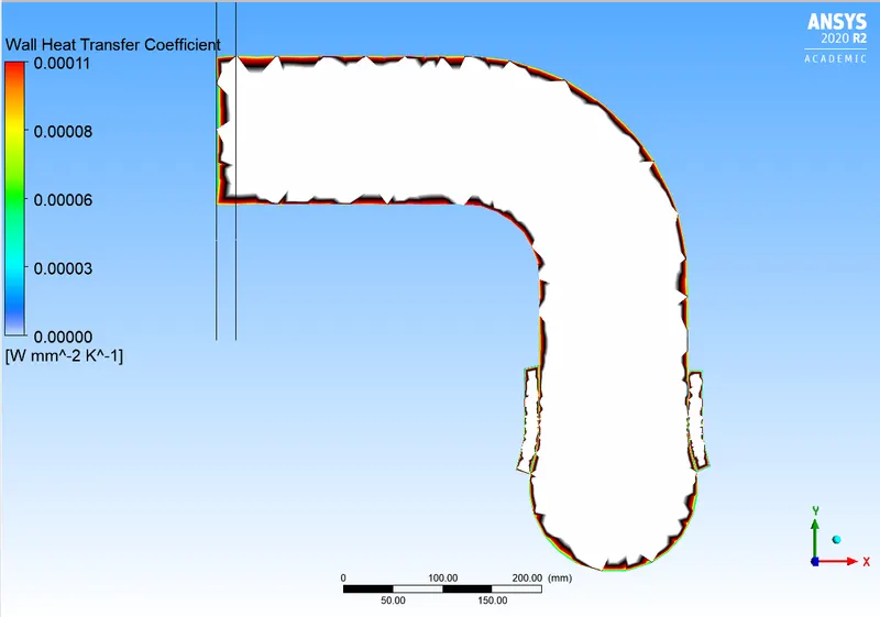
Fig 9. Wall heat transfer coefficient for run 1

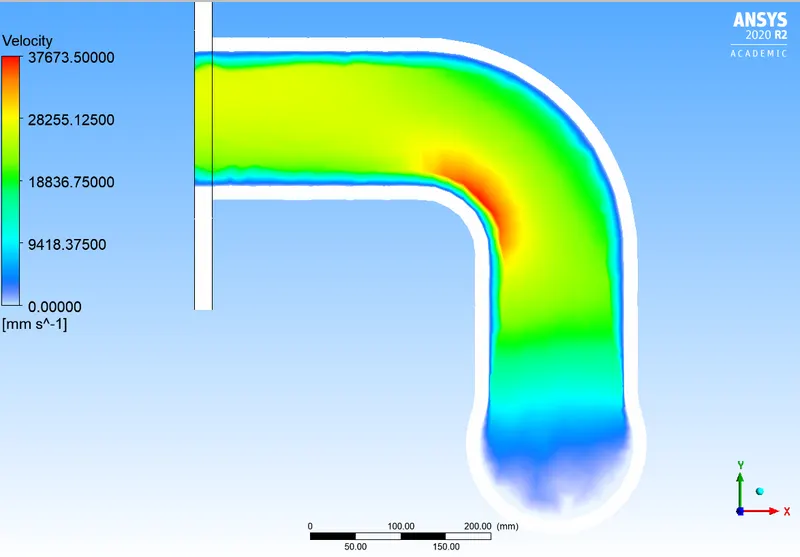
Fig 10. Velocity plane normal to Z for run 1

2) For run 2

No of elements = 247937

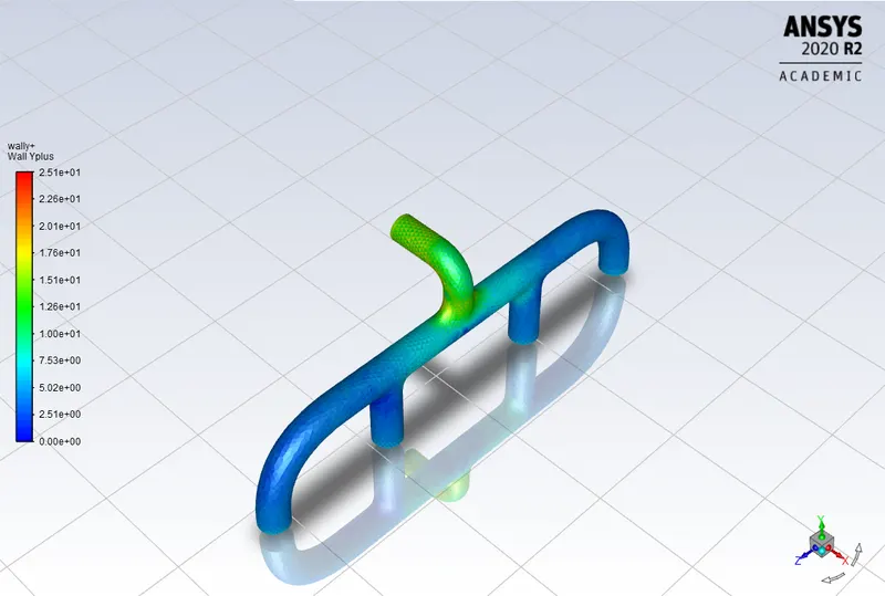
Fig 11. y+ value for run 2

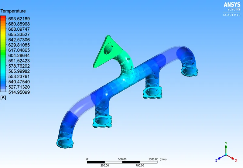
Fig 12. Temperature contours for run 2

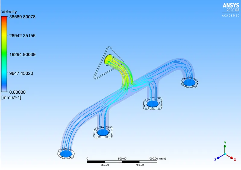
Fig 13. Velocity contours for run 2

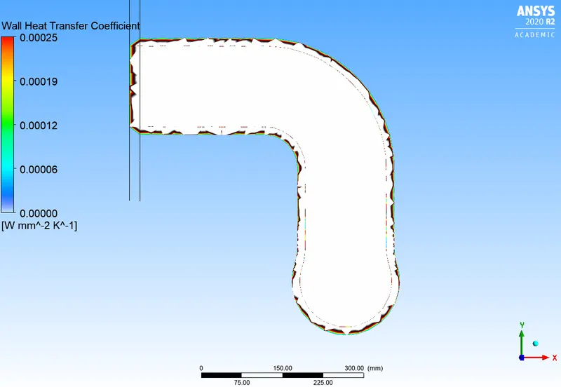
Fig 14. Wall heat transfer coefficient for run 2

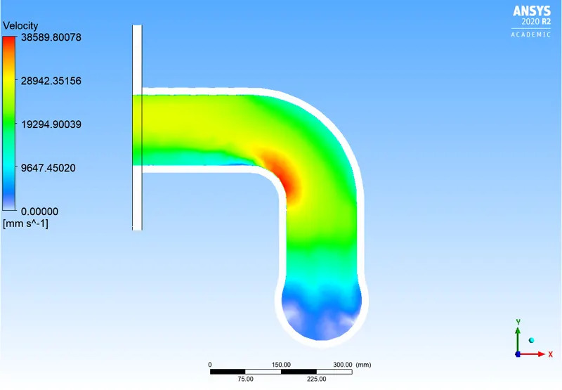
Fig 15. Velocity plane normal to Z-axis for run 2

3) For run 3

No of elements = 373813

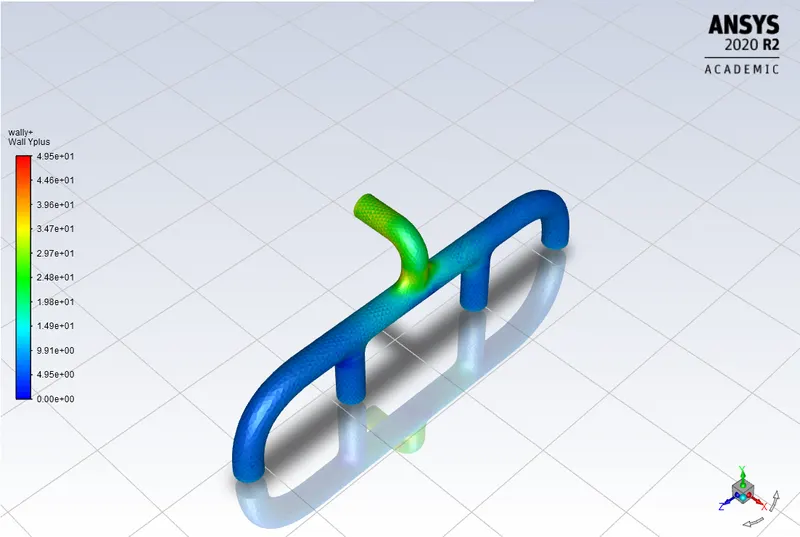
Fig 16. y+ value for run 3

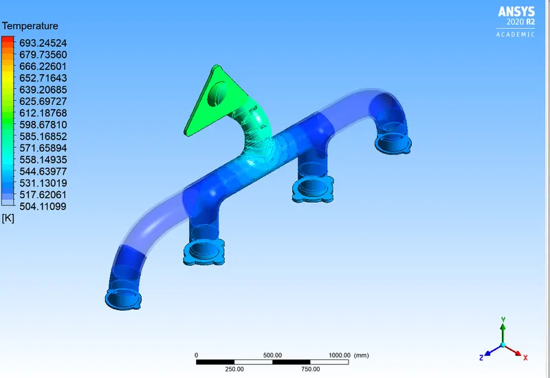
Fig 17. Temperature contour for run 3

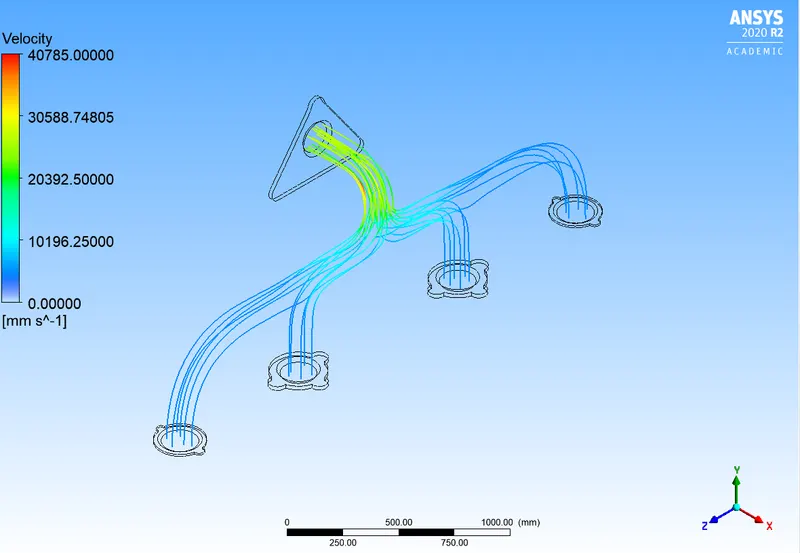
Fig 18. Streamlines for run 3

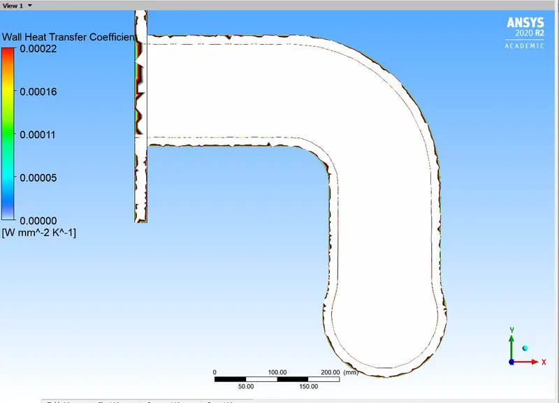
Fig 19. Wall heat transfer coefficient for run 3

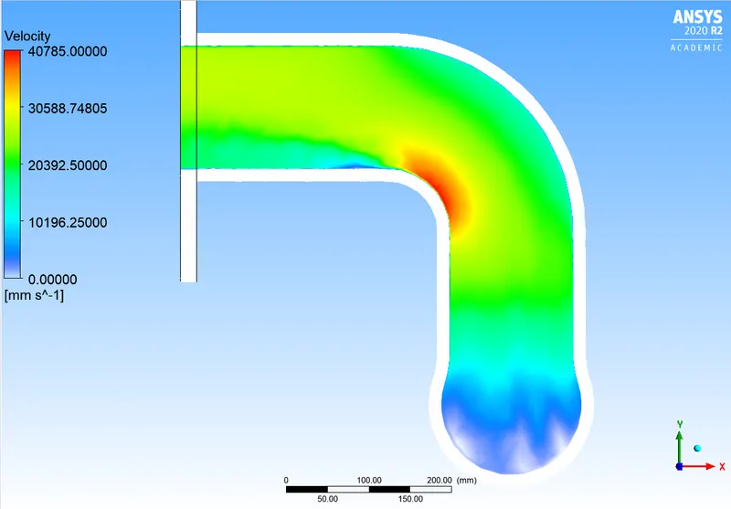
Fig 20. Velocity plane normal to Z for run 3

Inferences made:

Following are the inferences made from these runs.

1) Usually the wall y+ values for k-e turbulence theory are taken between 30 and 300. Meaning if the y+ value is less than 30 in a certain grid, we can make it a little bit coarser, and similarly if the

y+ value exceeds 300 we need to refine the grid there. As we can observe that in run 1, the maximum value is as high as 546. This is because the mesh is coarse and no inflation layer has been employed to it.

Similarly, on applying an inflation layer of 2.5 mm all around the walls the wall y+ value dropped to as low as 25. This is way too finer and this can be readjusted. So, in the third run, and inflation layer of 5 mm thickness is considered by applying a body sizing of 10 mm on solid volume. In this case, the maximum y+ value is 49.5 and it is well within the required range.

2) Better y+ values help in understanding the boundary layer phenomenon over the walls and this helps in understanding the heat transfer properly.

3) As we can observe that the location where there is a higher magnitude of wall heat transfer coefficient we observe a spike in velocity. This happens because higher the heat transfer coefficient, higher the Reynolds number, and therefore higher velocity.

Verification of the simulation results

In order to ensure whether the simulation results are correct, it should be compared with the theoretical correlations of the heat transfer or by conducting experiments mimicking the boundary conditions.

Further runs on this simulation is not possible owing to the element limit. So, we can assume that the maximum possible velocity to be 40.785 m/sec with maximum wall heat transfer to be 220 W/m^2.K