Week 6 - CHT Analysis on a Graphics card

AIM:

Conduct a steady-state conjugate heat transfer study on a graphics card model.

OBJECTIVE:

Simulate by adjusting the velocity from 1 to 5 metres per second for at least three times and discussing the results.
Determine the processor's maximum temperature and heat transfer coefficients.
With relevant pictures and charts, demonstrate that the simulation has reached convergence.
Determine any possible hotspots in the model.

THEORY:

Conjugate heat transfer analysis is utilised for processes involving a wide range of temperatures in solids and fluids owing to thermal contact. The heating or cooling of a substance by the movement of air is a common example. Heat transfer is the exchange of heat between two bodies, and the rate of heat transfer is directly proportional to the temperature differential between them. Heat transmission in solids is normally caused by conduction, but heat transfer in fluids is caused by convection. The key to developing good coolers, heaters, or heat exchangers is efficiently mixing heat exchanges between solids and fluids. The most prevalent method for achieving increased heat transfers is forced convection. Combining convection with phase change (for example, liquid water to vapour phase transition) improves performance even more in specific situations.

Procedure

To get the desirable results we go through 3 major steps in the same sequel and based on the steps we followed during whole setup we got the results.

1. First of all, open the workbench
2. Drag the Fluid Flow (fluent) part in the Project schematic window
3. So, via going through Geometry option open the Space claim
4. Go to the open – new – go to geometry location – select open command
5. By following step 4 we will able to open the geometry in the space claim
6. Now choose the required volume from the whole geometry to do further process efficiently.
7. Check for any overlaps and the intersections that cause problem in the meshing.
8. After verifying the model and then close the window.
9. Now open Ansys Meshing and let the geometry upload.
10. Then firstly name all the parts of the model.
11. Then from the Tree right click on mesh and tap "Generate mesh"
12. Set the sizing of the meshing from its detail and then repeat the step 11.
13. After verifying the mesh, close the Ansys Meshing window.
14. Now open Ansys fluent window by clicking over ‘Setup’ and let the geometry upload.
15. For verifying the check click of ‘Checks’ option and see the results in console.
16. Go to the General and set the case accordingly as mentioned in the challenge
17. As we are dealing with temperature so mark the Energy option and chose the viscous flow option to define the fluid flow.
18. After this set the Boundary conditions.
19. Generated the graphs that we want to observe during the case run.
20. With this go to the results and create a plan in from the centre of the body and allow to show the velocity contour pattern over it during the case run time.
21. In addition to this, from ‘solving’ section also select animation for the same velocity contour.
22. The initialize the case
23. Set the total no. of iteration.
24. Click calculate to make simulation run
25. As the simulation completed close the tab and do the postprocessing as analyse the contours and plots.
26. For this select the plane slice that is situated in the centre of the geometry and over it we have to perform the contour analysis.
27. Close the tab after extracting useful results.
28. Save the case and cut the software.

Results:

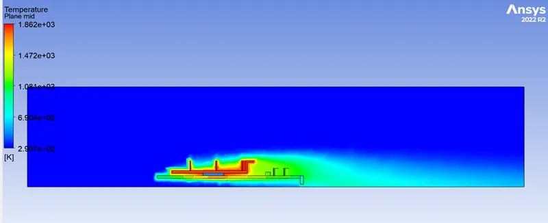
Rest of the all results are attached in the word file below.

Thanks

Anubhav