Conjugate Heat Transfer Analysis on a Graphics Card
A CHT or Conjugate Heat Transfer analysis is used where there are multiple phases in a simulation and energy transfer in the form of heat occurs between the multiple phases. An example could be a condenser of any type, where the hot working fluid transfers its heat energy to a coolant. A CHT analysis can be used to calculate the heat transfer coefficient of any part of the condenser system. Further examples include: cooling of an exhaust pipe, cooling of a computer graphics card and heating a moving fluid using a heating coil.
In this project, I will be simulating a system which involves cooling a computer graphics card that generates heat, the cooling process is simple, air at different velocities flow over the graphics card, which has fins to dissipate more heat.
Geometry
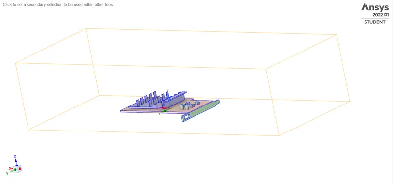
The geometry for this project was an .stl file which was imported into spaceclaim, the geometry consists of a base, processor, fins and external enclousure. The multiple components of the geometry have to be merged so that a body fitted mesh can be generated later, this is done by selecting FFF under Structure -> Analysis and set Share Topology to Share. Then, go to Workbench -> Share to start the sharing process. After this process is complete, the geometry is ready for meshing.
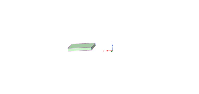
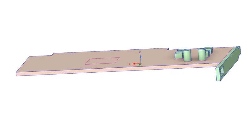
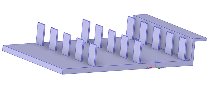
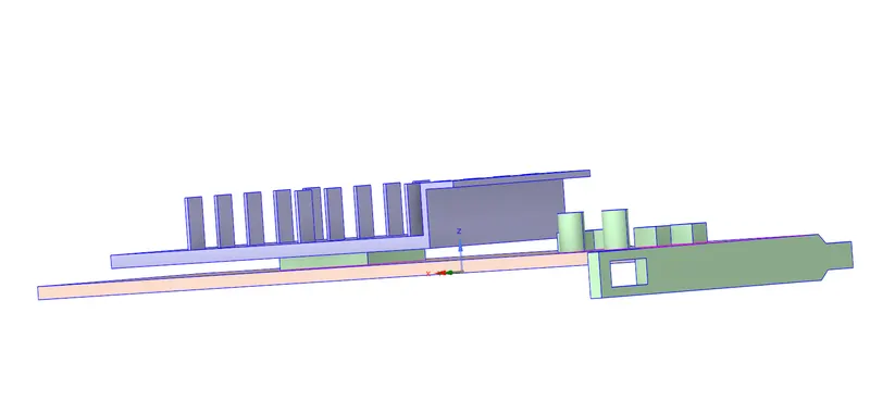
Pictures of each component are below:
1. Processor
2. Base
3. Fins
4. Base + Processor + Fins
5. Transparent Enclosure
Meshing
The meshing is done using ANSYS's Mechanical APDL.
The base mesh size is 5mm
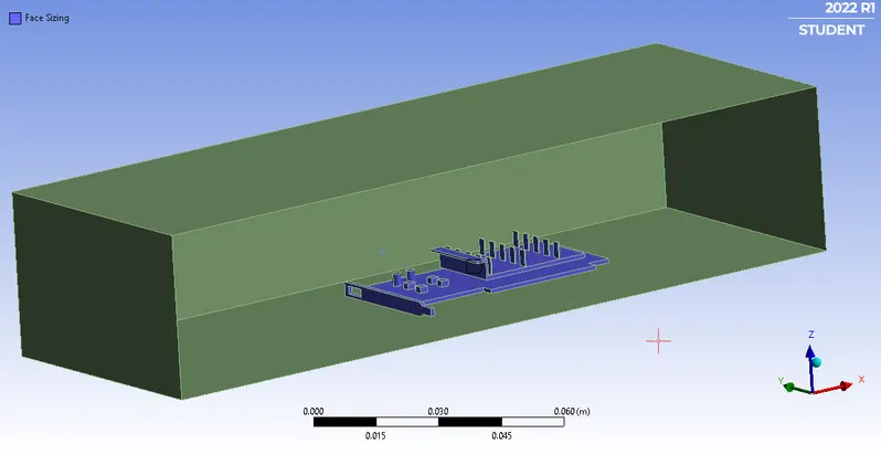
An additional control was included to improve the size of mesh in the regions near the graphics card. This improvement is to utilise more computational resources to finely generate temperature and velocity data after the simulation.
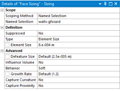
Controls -> Face Sizing -> Named Selection -> walls-gfxcard
This is where the body sizing has been applied (front enclousure wall hidden)
This is the final mesh on a sectional plane roughly across the axis:
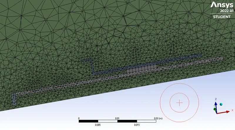
Zooming in,
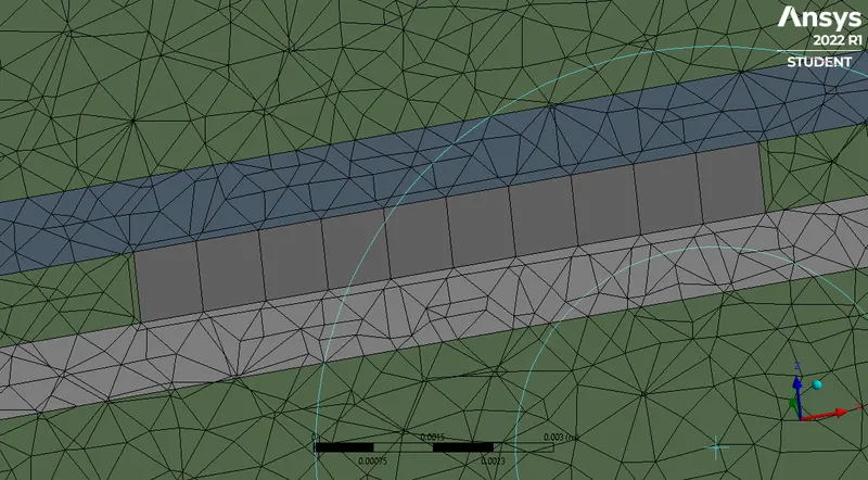
The mesh is conformal, this ensures simulation data is accurately transfered between different parts of the geometry.
The mesh metrices indicate that most of the elements have a quality greater than 0.6, which makes the quality satisfactory.
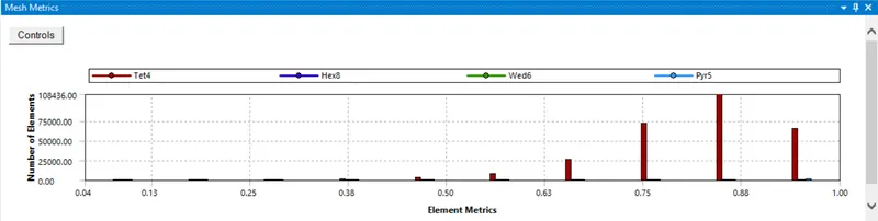
The mesh has 50529 nodes and 285011 elements.
Setup
Materials
The existing materials' properties were used and were left unchanged.
These were the materials used and its properties:
Density of Air: 1.225kg/m3">1.225kg/m3
Specific Heat of Air: 1006.43J/kg.K">1006.43J/kg.K
Thermal Conductivity of Air: 0.0242W/m.K">0.0242W/m.K
Viscosity of Air: 1.7894⋅10-5kg/m.s">1.7894⋅10−5kg/m.s
Density of Aluminium: 2719kg/m3">2719kg/m3
Specific Heat of Aluminium: 871J/kg.K">871J/kg.K
Thermal Conductivity of Aluminium: 202.4W/m.K">202.4W/m.K
Density of Gold: 19320kg/m3">19320kg/m3
Specific Heat of Gold: 129.81J/kg.K">129.81J/kg.K
Thermal Conductivity of Gold: 297.73W/m.K">297.73W/m.K
Density of Titanium: 4850kg/m3">4850kg/m3
Specific Heat of Titanium: 544.25J/kg.K">544.25J/kg.K
Thermal Conductivity of Titanium: 7.44W/m.K">7.44W/m.K
Boundaries
inlet - inlet velocity of 1m/s, 2.5m/s and 5m/s normal to the boundary
outlet - pressure outlet
other surfaces were left unchanged, some were wall and others were interior.
Cell Zones
This step is very important as it lets ANSYS know which regions consists of fluid flow (convection) and which regions consist of solid (conduction)
enclousure - fluid - air
base - solid - titanium
processor - solid - gold
fins - sold - aluminium
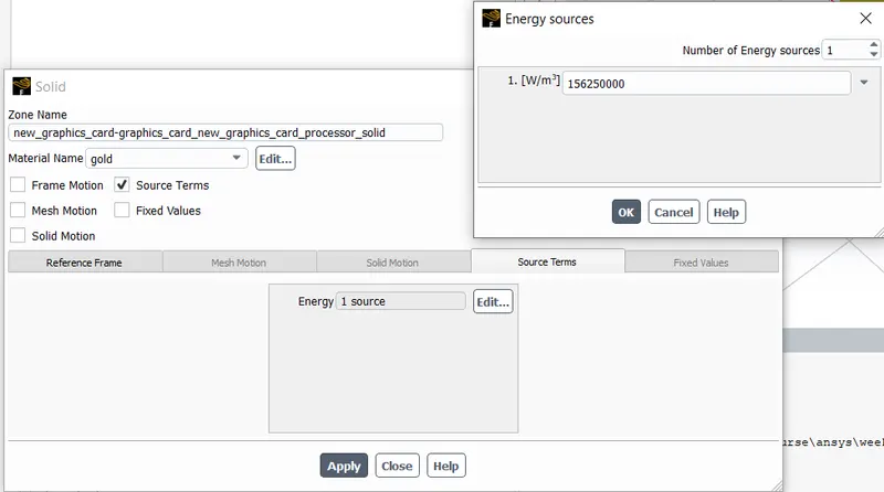
The condition that the processor generates heat was also given in this step, the processor was assumed to emit 10W. The input field required the heat to be in W/m3">W/m3, hence the volume of the processor was calculated using SpaceClaim.
Dimensions of cubiodal processor: 8mm×8mm×1mm">8mm×8mm×1mm
Volume of cubiodal processor: 64×10-9mm3">64×10−9mm3
Heat generated in W/m3">W/m3 : 10/(64×10-9)=156230000W/m3">10/(64×10−9)=156230000W/m3
Viscous
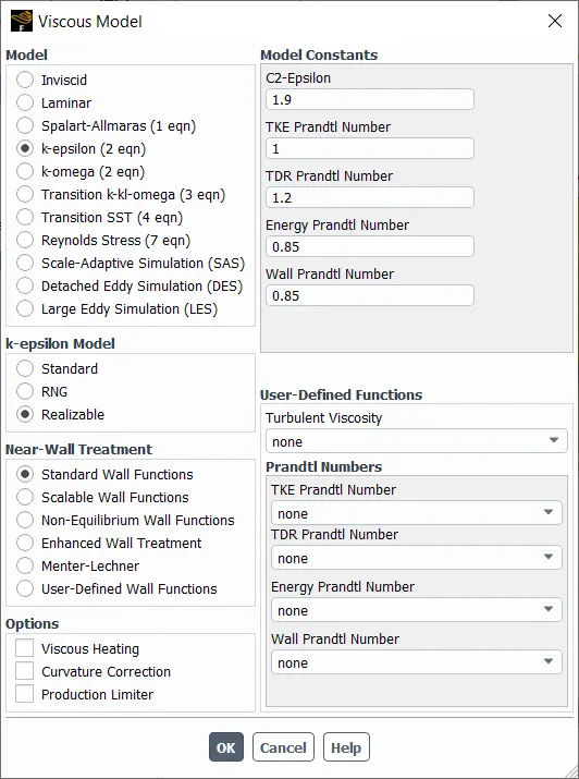
k-epsilon standard with standard near wall treatment was the viscous model used.
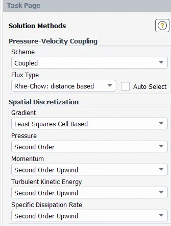
Solution - Methods
Simulation Results
The simulation ran until residuals dropped below 10^-3 using the steady state solver and with a hybrid initialisation. The results are below:
Inlet Velocity: 1m/s
Residuals
This was taken in ANSYS Fluent.
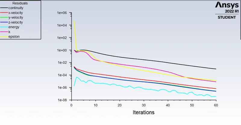
The simulation is said to be converged because of the extremely low residuals, even a further decrease in residuals will not alter the final temperature in a significant way.
Cut plane view of temperature
This was taken in CFD-Post.
A plane was created along the XZ plane at Y = 0, and the temperature contours were plotted
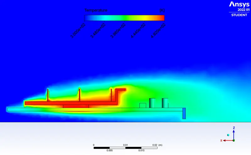
Maximum Processor Temperature: 492K">492K
Heat Transfer Coefficient of the Fin: 829.19WKm2">829.19WKm2
Inlet Velocity: 2.5m/s
Residuals
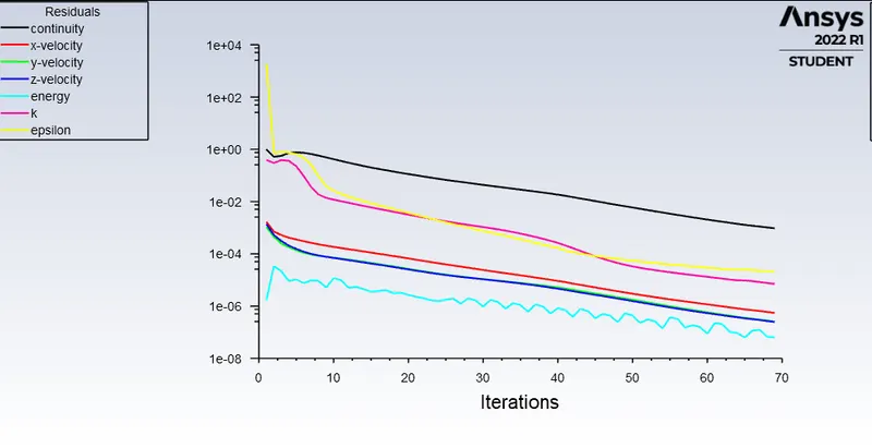
The simulation is said to be converged because of the extremely low residuals, even a further decrease in residuals will not alter the final temperature in a significant way.
Cut plane view of temperature
This was taken in CFD-Post.
A plane was created along the XZ plane at Y = 0, and the temperature contours were plotted
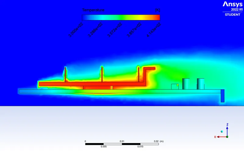
Maximum Processor Temperature: 414K">414K
Heat Transfer Coefficient of the Fin: 1089.5WKm2">1089.5W/Km2
Inlet Velocity: 5m/s
Residuals
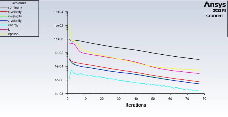
The simulation is said to be converged because of the extremely low residuals, even a further decrease in residuals will not alter the final temperature in a significant way.
Cut plane view of temperature
This was taken in CFD-Post.
A plane was created along the XZ plane at Y = 0, and the temperature contours were plotted
Maximum Processor Temperature: 378.86K">378.86K
Heat Transfer Coefficient of the Fin: 1310.44WKm2">1310.44W/Km2
Hotspots
These were taken in CFD-Post.
This shows the regions were temperature is higher than its surroundings:
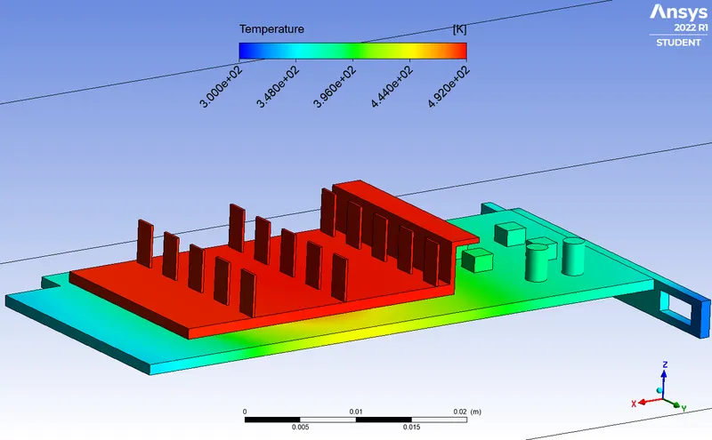
The temperature is higher in the fins because of easy conduction of heat between processor and fins. Also, a lot of heat is dissipated through the fins, which enables the fins to accept more heat.
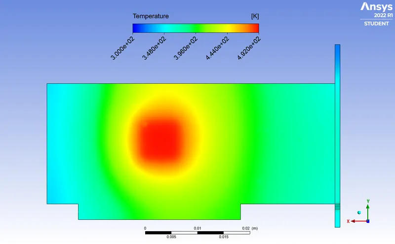
A hotspot is noticed at the bottom of the base, below where the processor fits. Heat is concentrated because of lower thermal conductivity of the base, and because there is less heat transfer due to convection.
Observations and Conclusions
1. The heat transfer coeffcient increases as velocity increases, this is an expected qualitative result because there is more air to absorb heat when the velocity is high.
2. The highest temperature on the processor also decreases as velocity of cooling air increases. This is because the increase in heat transfer coefficients.
3. Hotspots were observed at two regions near the processor and the reasons for the accumulation of heat were explained.