Week 6 - CHT Analysis on a Graphics card
REPORT FOR CHALLENGE-6:
Aim : To perform the steady-state conjugate heat transfer analysis on a garphic Card for to find the convective heat transfer, maximum and average temperatures due to the fluid passing externally over the graphic card with the velocities of 1, 3 and 5m/s undar the ambient temperature conditions in coarse and fine element cases.
Software Required : Ansys Workbench – Fluid Flow vR2-2022
Hardware Required : Desktop, Keyboard, Mouse, CPU.
Theory:
Conjugate heat transfer corresponds with the combination of heat transfer in solids and heat transfer in fluids. In solids, conduction often dominates whereas in fluids, convection usually dominates. Conjugate heat transfer is observed in many situations. For example, heat sinks are optimized to combine heat transfer by conduction in the heat sink with the convection in the surrounding fluid.Conjugate heat transfer model was developed after computers came into wide use in order to substitute the empirical relation of proportionality of heat flux to temperature difference with heat transfer coefficient which was the only tool in theoretical heat convection since the times of Newton. This model, based on a strictly mathematically stated problem, describes the heat transfer between a body and a fluid flowing over or inside it as a result of the interaction of two objects. The physical processes and solutions of the governing equations are considered separately for each object in two subdomains. Matching conditions for these solutions at the interface provide the distributions of temperature and heat flux along the body–flow interface, eliminating the need for a heat transfer coefficient.
Reynolds number (Re): It is a dimensionless quantity that helps predict fluid flow patterns in different situations by measuring the ratio between inertial and viscous forces. At low Reynolds numbers, flows tend to be dominated by laminar flow, while at high Reynolds numbers flows tend to be turbulent. The turbulence results from differences in the fluid's speed and direction, which may sometimes intersect or even move counter to the overall direction of the flow.
The Prandtl number is a dimensionless quantity that puts the viscosity of a fluid in correlation with the thermal conductivity. It therefore assesses the relation between momentum transport and thermal transport capacity of a fluid. It is defined as
Pr=Thermal (or heat) transport/Momentum transport=α/ν
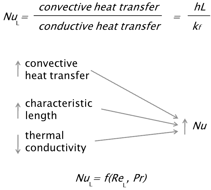
The Nusselt number(Nu) is a dimensionless number, is equal to the dimensionless temperature gradient at the surface, and it provides a measure of the convection heat transfer occurring at the surface.Thus, the Nusselt number is defined as:
Fin : A fin is a surface that extends from an object to increase the rate of heat transfer to or from the environment by increasing convection. Adding a fin to an object increases the surface area and can sometimes be an economical solution to heat transfer problems. Finned surfaces are commonly used in practice to enhance heat transfer. In the analysis of the fins, we consider steady operation with no heat generation in the fin. We also assume that the convection heat transfer coefficient h to be constant and uniform over the entire surface of the fin. The rate of heat transfer from a solid surface to atmosphere is given by Q = hA ∆ T where, h and ∆T are not controllable. So, to increase the value of Q surface area should be increased. The extended surface which increases the rate of heat transfer is known as fin.
Procedure :
1.Open the Ansys Workbench.
2.Double click or drag the Fluid Flow module.
3.Import the required geometry and extract the volume by selecting the required edges and to share topology for the common node points.
4.Mesh the geometry with the suitable element size in addition to name all the faces which model have.
- Provide the sizing for to assign the fine mesh for the fluid.
- Assign the Names for all the faces.
5.Solve the equations in the set-up and solution block for required result.
- Set 3D, Double Precision and Assign number of cores.
- Set Steady state.
- Change method to Coupled.
- Set Energy on and choose the K-Omega Turbulance model.
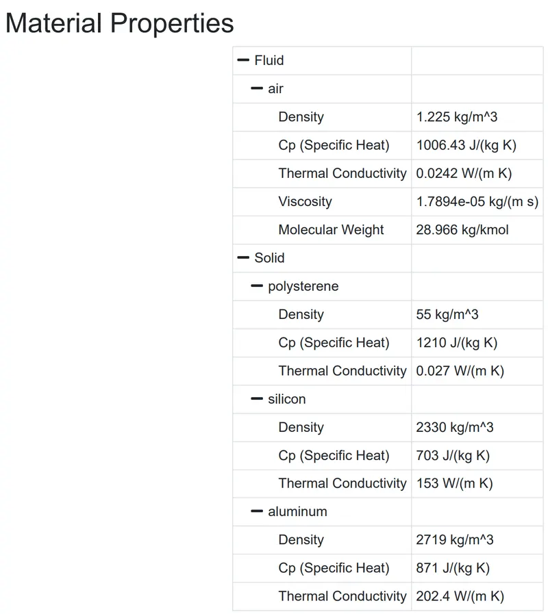
- Assign the Materials.
- Set fluid as air.
- Set solid and create three different suitable solid materials(eg.silicon,aluminum,polysteryne) along with their properties for to assign to the various parts in the processor.
- Assign the materials to the cell zones as shown-
- Set fluid as fluid and the material is air.
- Set the graphic card as solid and the material is silicon.
- Set the fins as solid and the material is aluminium.
- Set the pcb as solid and the material is polysterene.
- Assign the heat flow rate dissipated by the graphic card.
- Assign the Boundary conditions such as velocity and required temperature.
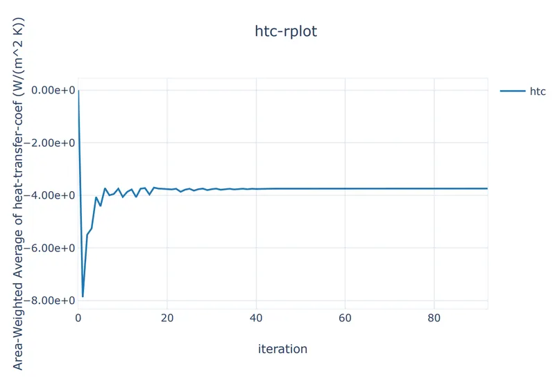
- Create definition plots for htc, tavg and tmax for graphics card.
- Create a plane and contours for temperature.
- Initialize and Calculate.
6.Then do the post-processing in the CFD solver in the result block.
7.Save and close the file.
Observations :
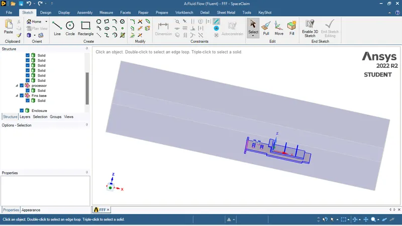
Geometry:
-Model to be Analize after Cad clean-up.
Mesh Details:
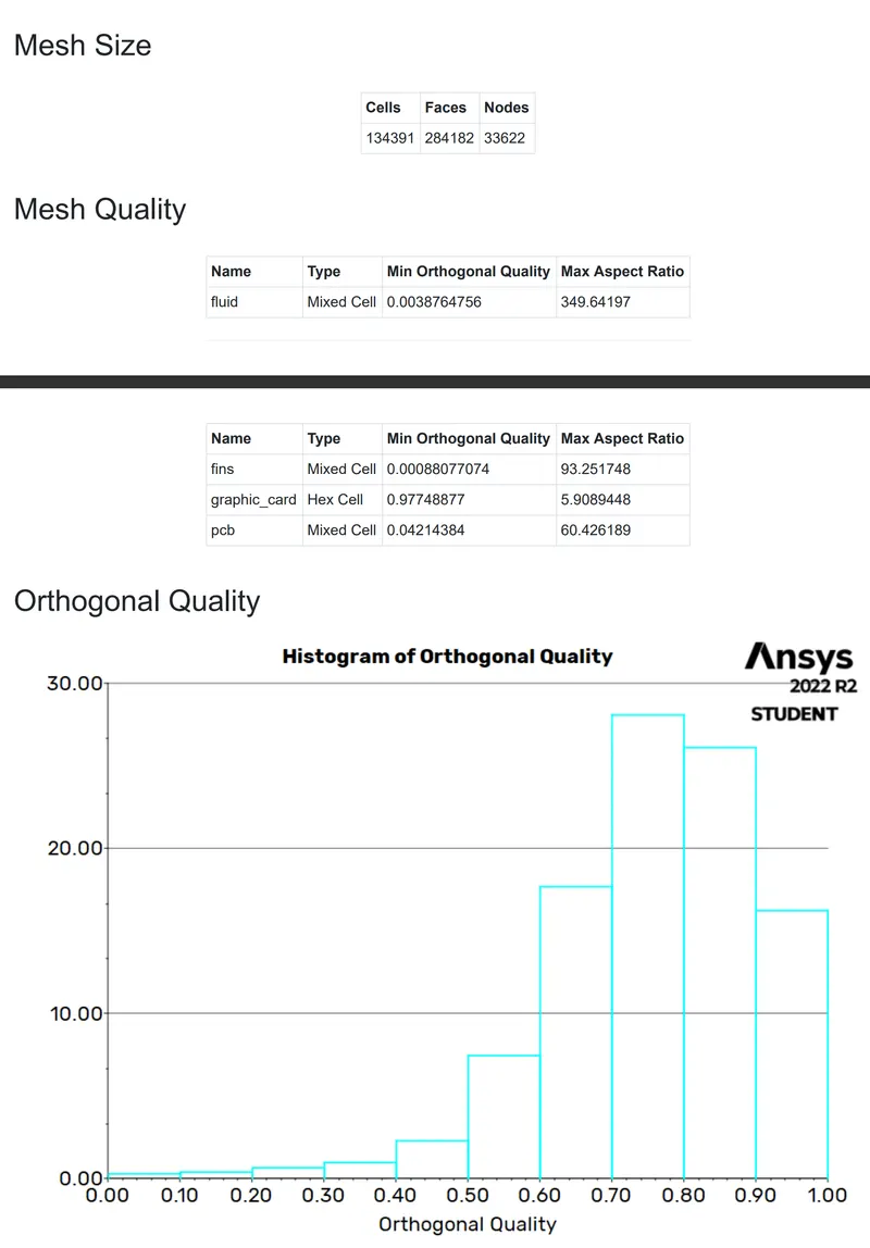
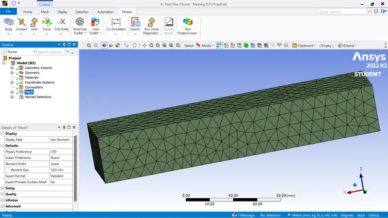
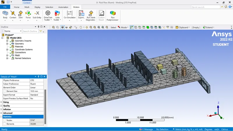
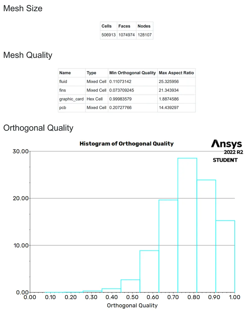
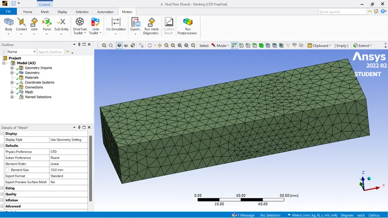
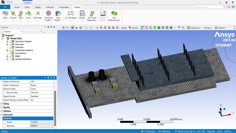
On the consideration of the accuracy of the result, we worked on the concept of independent grid generation. So, we analysed the given exhaust port in 2 different cases which are Medium and Fine mesh and all the mesh details were given below,
1.Coarse Mesh:
2.Fine Mesh:
Cell-Zone Conditions:
| fluid | fluid(air) |
| fins | solid(Aluminium) |
| graphic-card |
solid(Silicon)
|
| pcb | solid(polysterene) |
Materials:
Boundary Conditions:
| Mesh Type | Velocity(m/s) |
| Coarse | 1 |
| 3 | |
| 5 | |
| Fine | 1 |
| 3 | |
| 5 |
Solution Status:
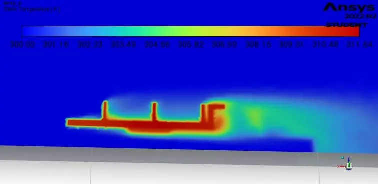
We analyzed the given body in 3 different velocity cases for 2 different element count each. The details were given below,
Coarse Mesh:
Case-1:V=1m/s
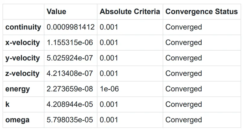
-After the required equations solved, tabulated the results that were obtained.
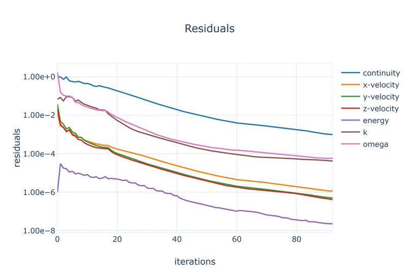
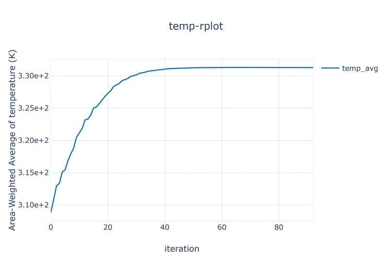
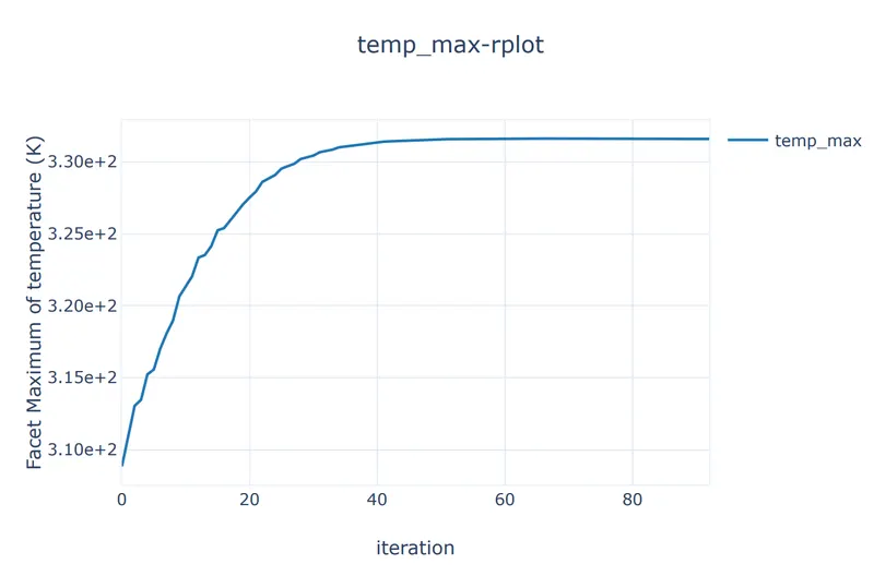
-Solution Converged at 93 iteration.
Plots and Contours:
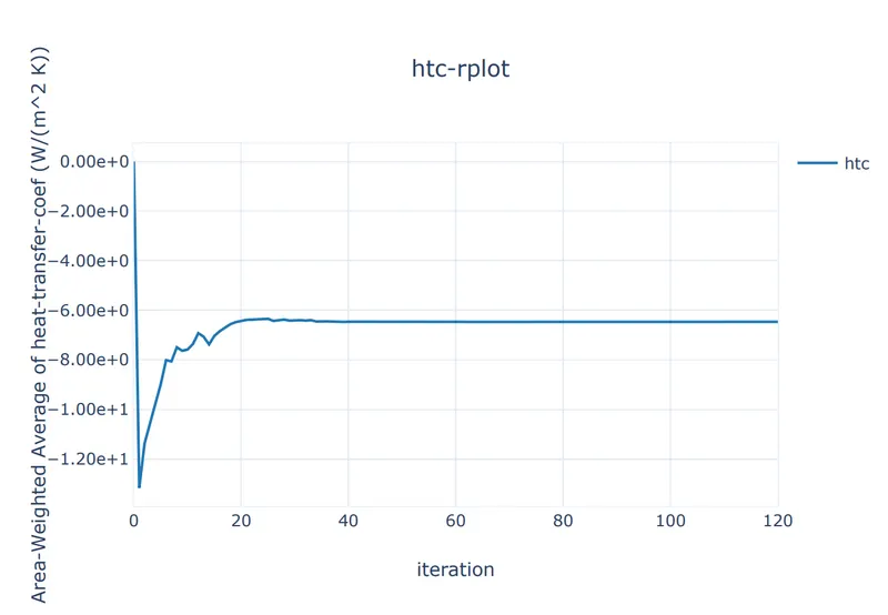
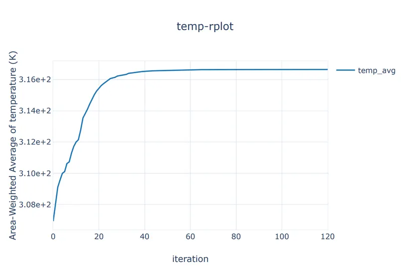
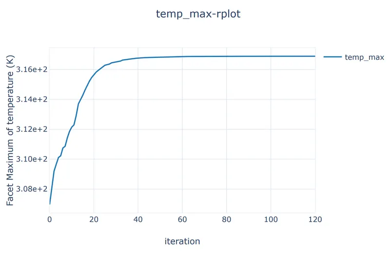
Case-2:V=3m/s
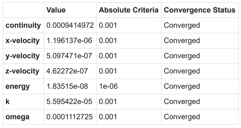
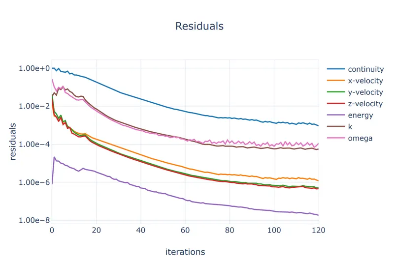
-After the required equations solved, tabulated the results that were obtained.
-Solution Converged at 121 iteration.
Plots and Contours:
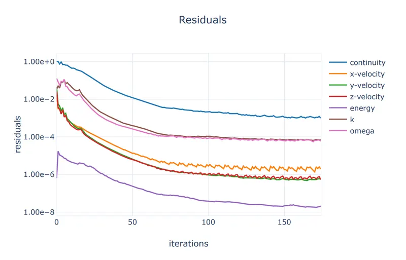
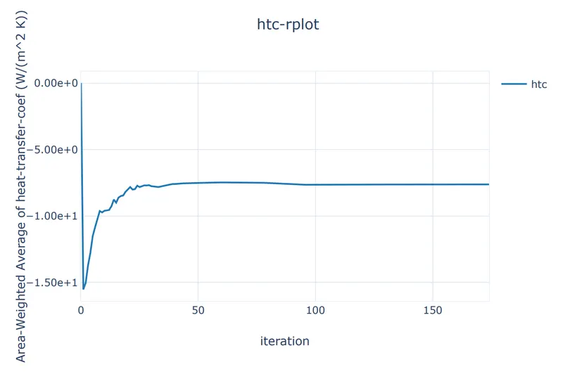
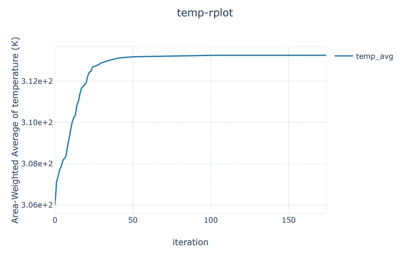
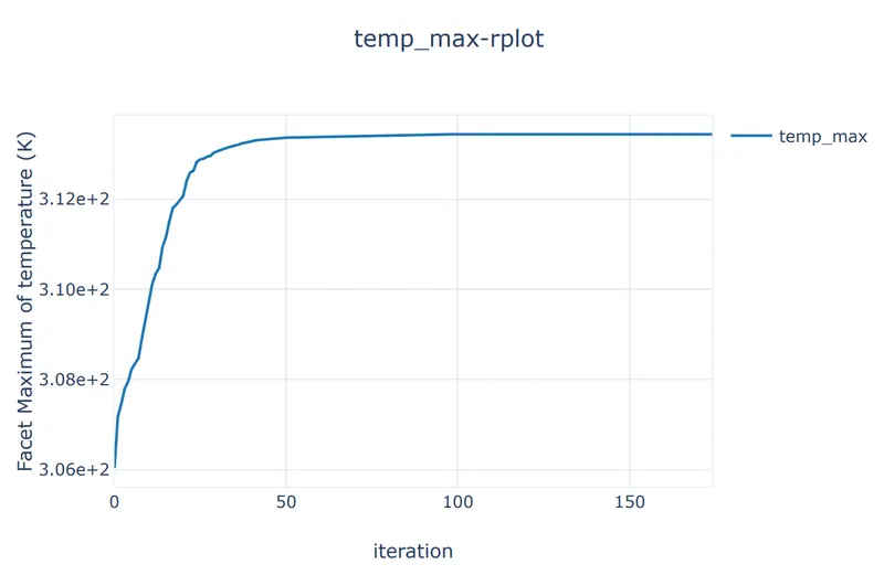
Case-3:V=5m/s
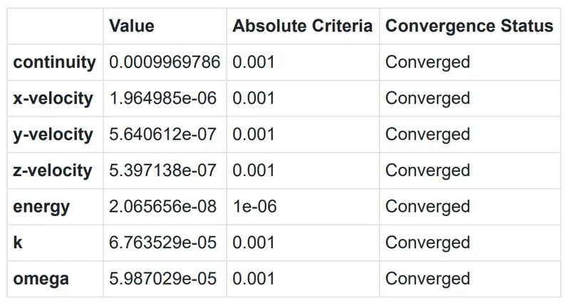
-After the required equations solved, tabulated the results that were obtained.
-Solution Converged at 175 iteration.
Plots and Contours:
Fine Mesh:
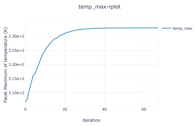
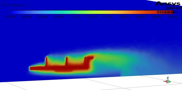
Case-1:V=1m/s
-After the required equations solved, tabulated the results that were obtained.
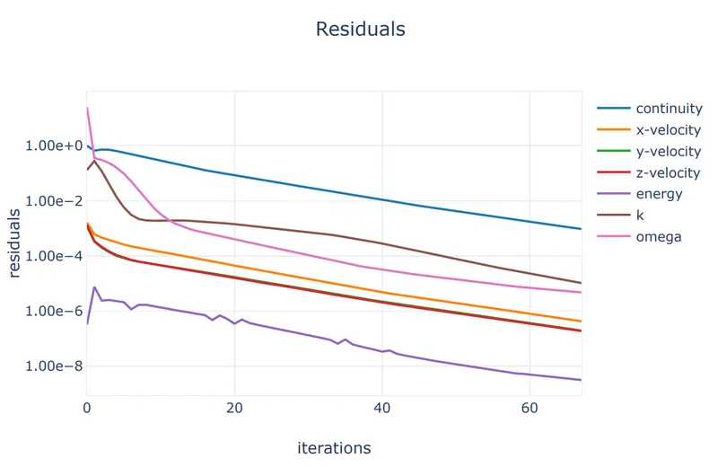
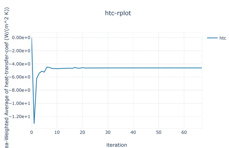
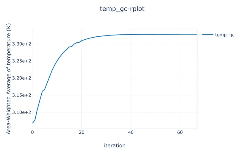
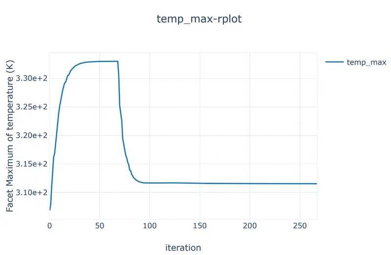
-Solution Converged at 68 iteration.
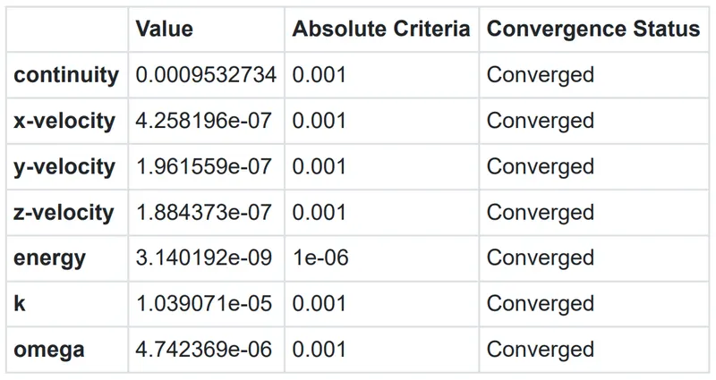
Plots and Contours:
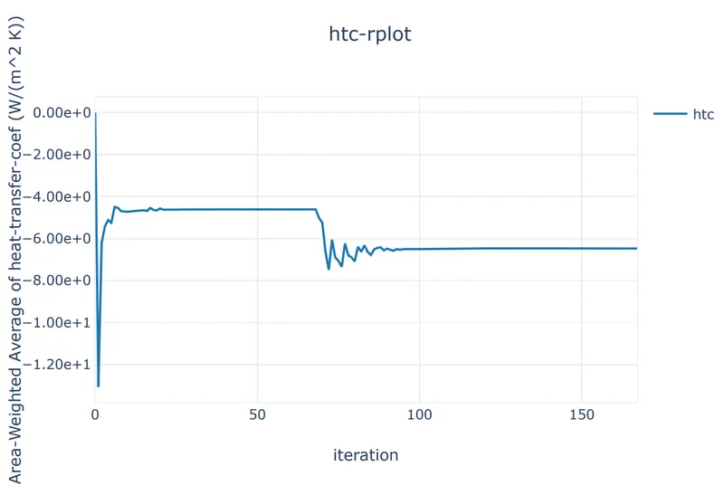
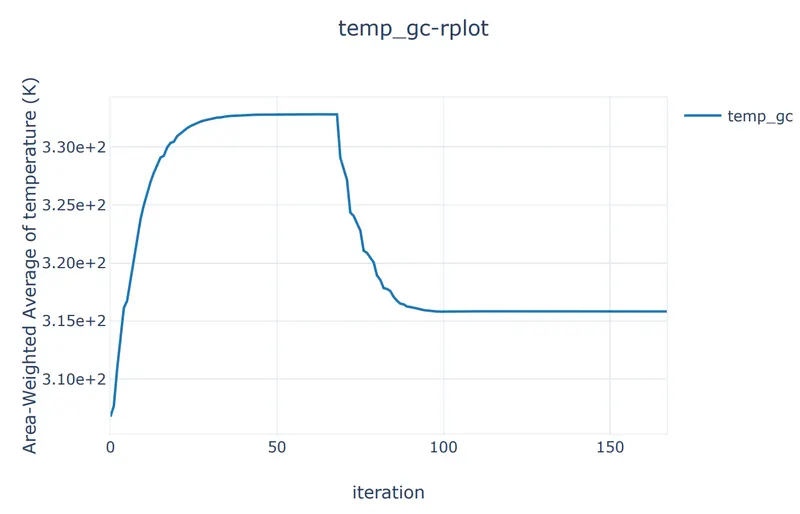
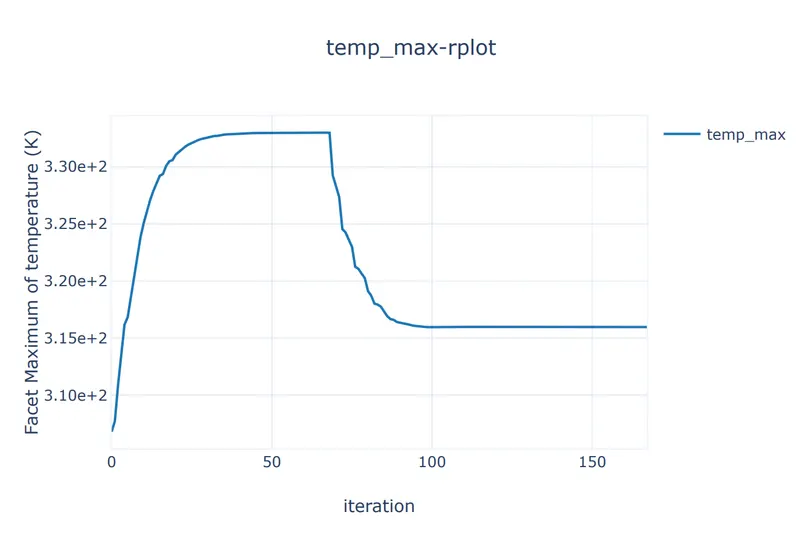
Case-2:V=3m/s
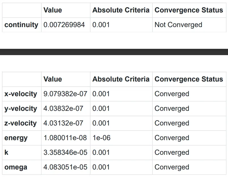
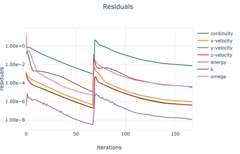
-After the required equations solved, tabulated the results that were obtained.
-Solution Converged at 168 iteration.
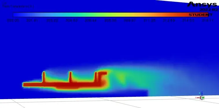
Plots and Contours:
Case-3:V=5m/s
-After the required equations solved, tabulated the results that were obtained.
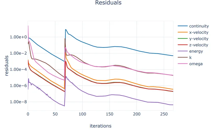
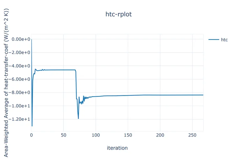
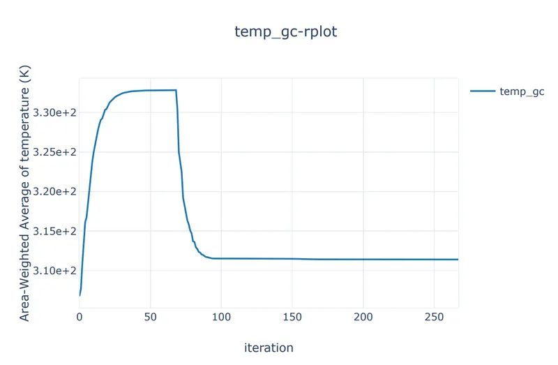
-Solution Converged at 300+ iteration.
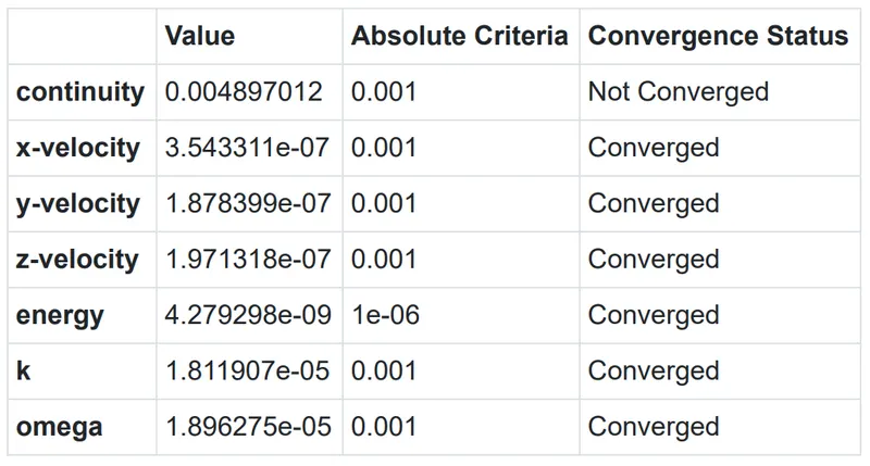
Plots and Contours:
Precautions :
1.Carefully solve the problem.
2.Choose the suitable methods carefully for to get the desired results.
3.Note down the values carefully which are required for theoretical calculations.
Result:
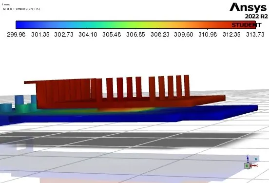
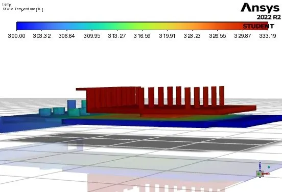
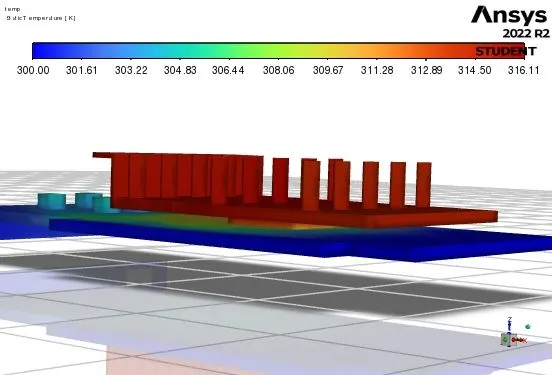
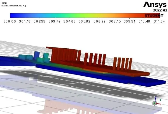
Convective heat transfer coefficients for 2 different meshes were given below,
| Case | No.of elements | Velocity(m/s) | h-gc(W/m^2-k) | T-gc-avg(k) | T-gc-max(k) |
| 1 | 3.7417 | 331.27 | 331.58 | ||
| Medium | 1,34,391 | 3 | 6.4642 | 316.64 | 316.88 |
| 5 | 7.6211 | 313.24 | 313.43 | ||
| 1 | 4.6115 | 332.81 | 332.97 | ||
| Fine | 5,06,913 | 3 | 6.4766 | 315.83 | 315.97 |
| 5 | 8.3740 | 311.40 | 311.52 |
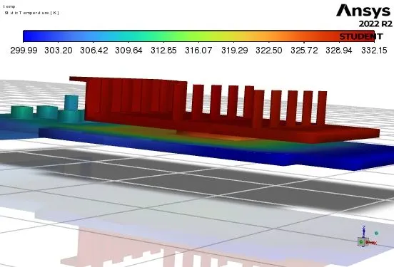
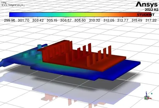
Contours for all cases:
Coarse:
1.V=1m/s
2.V=3m/s
3.V=5m/s
Fine:
1.V=1m/s
2.V=3m/s
3.V=5m/s
Conclusion:
Heat transfer in solids and heat transfer in fluids are combined in the majority of applications. This is because fluids flow around solids or between solid walls, and because solids are usually immersed in a fluid. An accurate description of heat transfer modes, material properties, flow regimes, and geometrical configurations enables the analysis of temperature fields and heat transfer. Such a description is also the starting point for a numerical simulation that can be used to predict conjugate heat transfer effects or to test different configurations in order, for example, to improve thermal performances of a given application.
It was observed that convective heat tranfer coefficient in either outer or inner walls increases with the increase of the renyolds number.
It seems that the average temperature and the maximum temperature of the graphics card is very close to each other. Also we can come to a colleague that the accuracy is always shows the difference in the size of the mesh element.