Week 6 - CHT Analysis on a Graphics card

Objective:

Perform a steady-state conjugate heat transfer analysis on a model of a graphics card. You can use appropriate materials of your choice for the simulation. Make sure to properly define the correct solid and fluid zones. Refer to the video for further clarification and the model is provided below the video.

Run the simulation for the best possible mesh with a combination of coarse and refined mesh in different regions. Explain the reason for choosing the particular mesh settings.

Aims:

1. Run the simulation by varying the velocity from 1m/sec to 5m/sec for at least 3 velocities and discuss the results.
2. Find out the maximum temperature and heat transfer coefficient attained by the processor.
3. Prove that the simulation has achieved convergence with appropriate images and plots.
4. Identify potential hotspots on the model.

Solution:

What is the conjugate heat transfer analysis in a system?

Conjugate heat transfer is a type of heat transfer analysis between solids and fluid(s). This type of heat transfer includes both convection (between fluids) and conductive (between solids) heat transfer, as well as both forced and natural convection. Common applications and use cases of this thermal simulation type include electronics cooling, heat exchangers, industrial machinery, some AEC cases, and more. In order to demonstrate best practices for this application type, an electronics cooling application will be used as an example.

Our project focuses on electronics cooling performance, as the CHT simulation type is most commonly used for this type of application. We will explain how to set up the analysis on the Ansys-FLUENT platform, what guidelines to follow to guarantee success, how to make sure our results are good, and how to make sure your solution is fully converged.

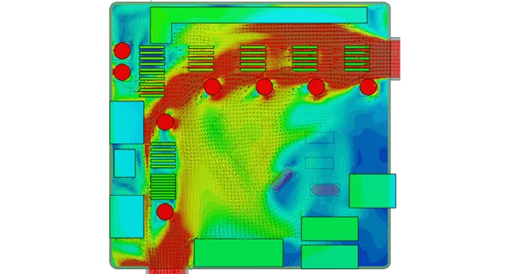
The above picture shows the heat flow over the heat sink in an inlet in an electronics circuit board. Mostly we use electrical appliances or systems.

we are going to set up a simulation where we are going to run it on the graphics processor unit GPU of a computer system. To investigate the conjugate heat transfer analysis for heat sinks that are being used in electronics cooling. This involves the combined fluid flow analysis by
making use of CFD equations and heat transfer analysis, considering separately convection process in fluid flow region and conduction heat transfer in the solid region.

To carry out heat transfer analysis for different fin configurations considering the conduction heat transfer from the base plate to heat fins.

3. To conduct computational fluid flow analysis for different fin configurations, for a fluid part, by solving Navier-Stroke equations to get velocity vectors, pressure contours, and temperature fields for given inlet air velocity. Any Standard RANS model is adopted to account for the turbulence phenomenon. The temperature field is used to get the quantity of heat dissipated or carried away by convection.

4. To determine the heat transfer coefficient, Thermal resistance, and Pressure drop through numerical to predict the thermal performance of a fin for different geometrical configurations.

5. To select the best heat sink with suitable fin geometry for lower thermal resistance, higher heat transfer coefficient, and minimum resistance.

Case 1:Inlet velocity 1m/s

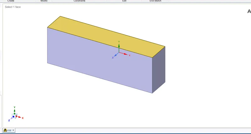
Model opened in spaceclaim

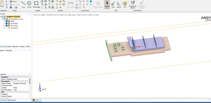
Showing fin base, fins and processor

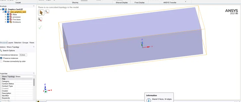
DONE SHARED TOPOLOGY

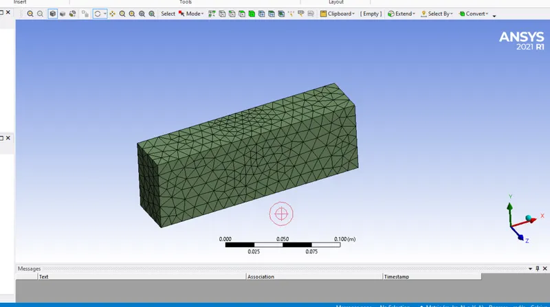
Meshing done with default mesh

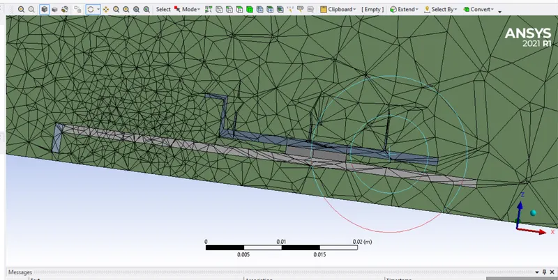
Confirmel mesh is formed

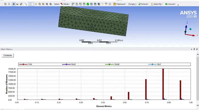
Quality of mesh checked

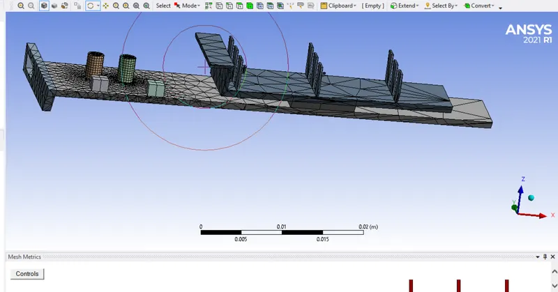
Showing mesh in internal parts

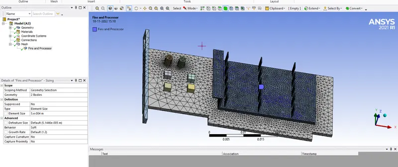
Given body sizing to fins and processors with 0.5mm mesh

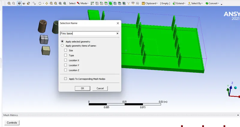
Giving naming to the parts

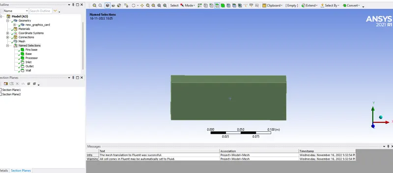
Given naming to all parts

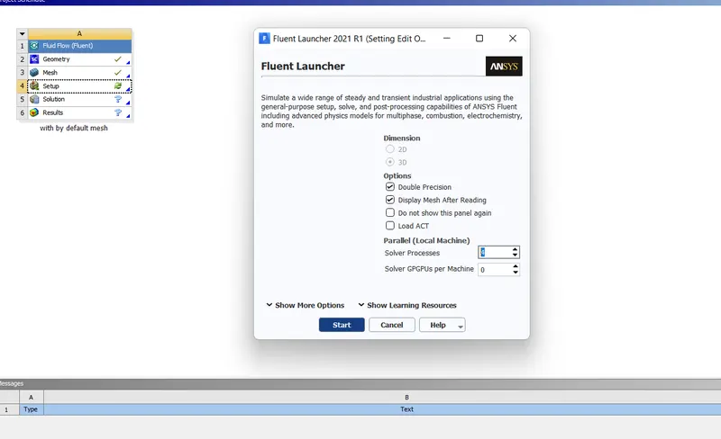
Opening setup window

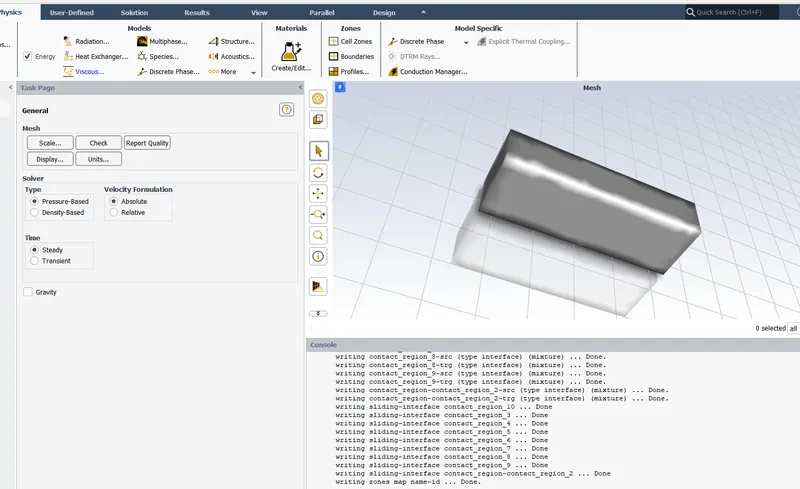
Given steady state condition and energy equation

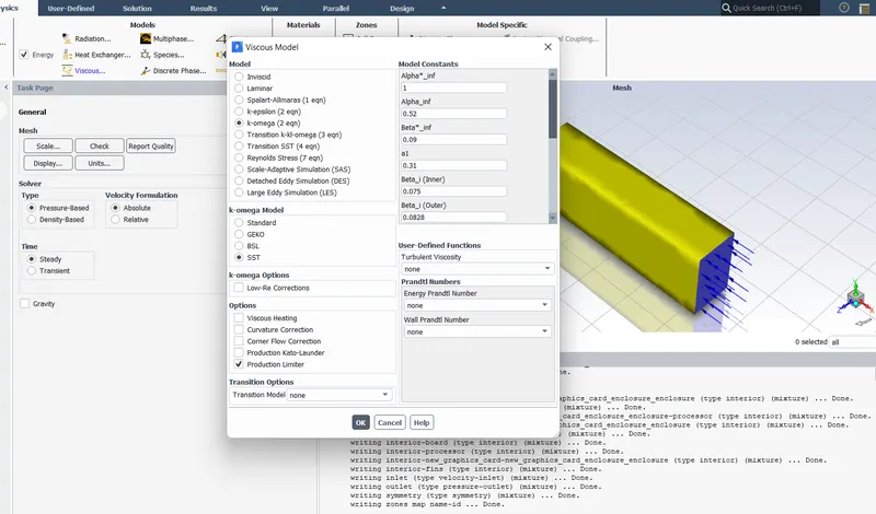
Giving K-Omega SST Model

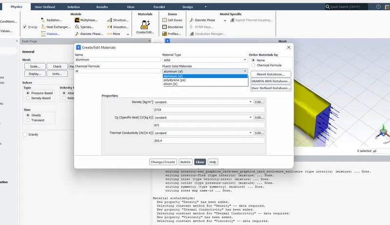
Material added

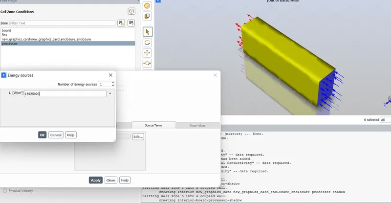
Giving heat source term to the processor

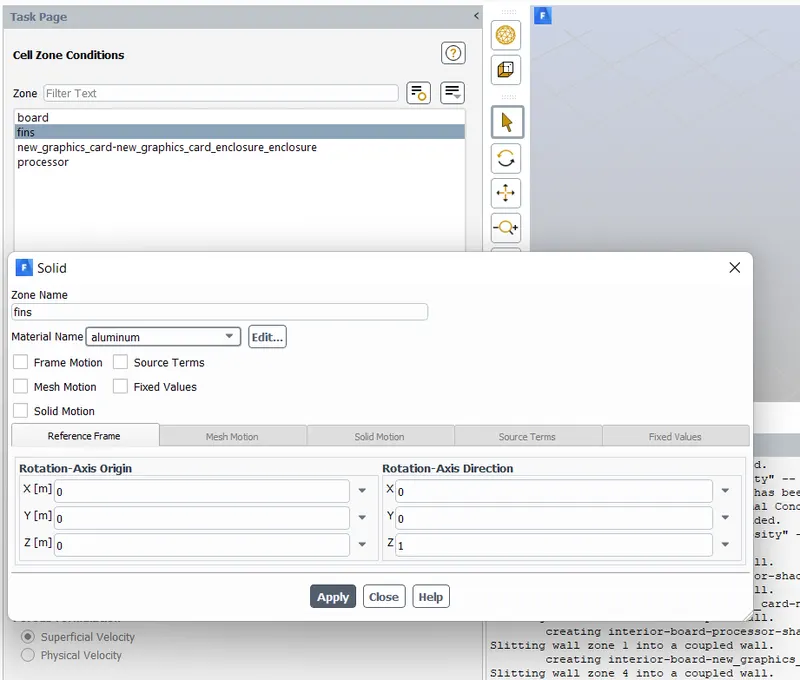
Assigning material to fins

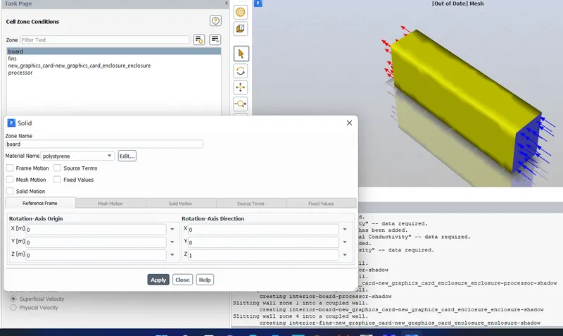
Assigning material to board

CASE 1:Inlet velocity 1m/s

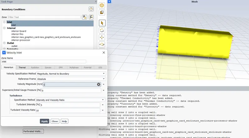
Giving inlet boundary conditions

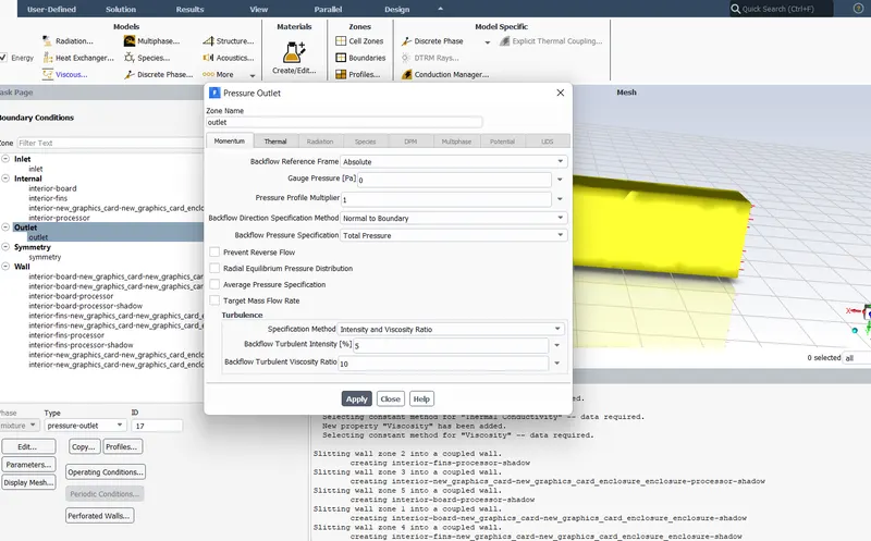
Giving outlet boundary conditions

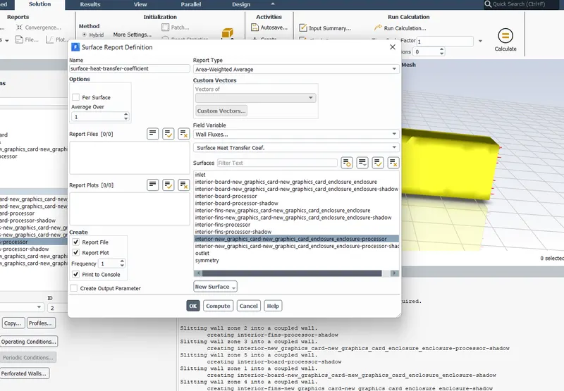
Setting area weighted average of surface heat transfer coefficient

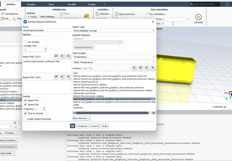
Setting area weighted average of average temeperature at the processor walls

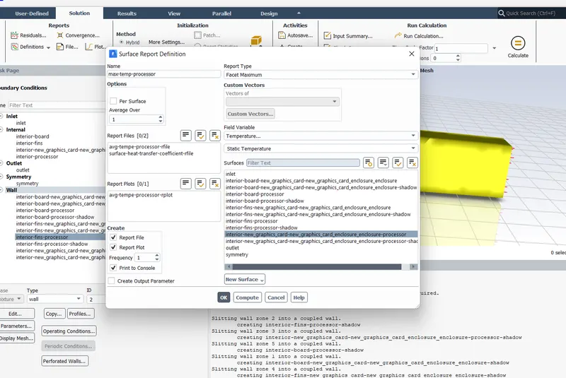
Setting maximum temperature at the processor walls

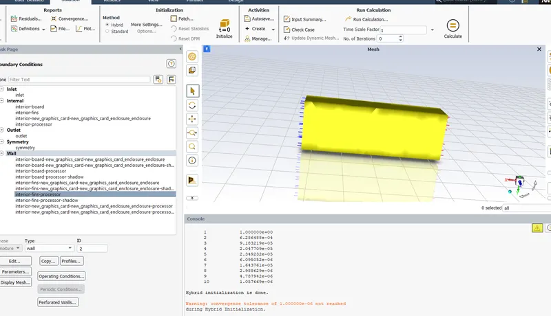
Hybrid Initialization done

RESULTS AND DISCUSSIONS:

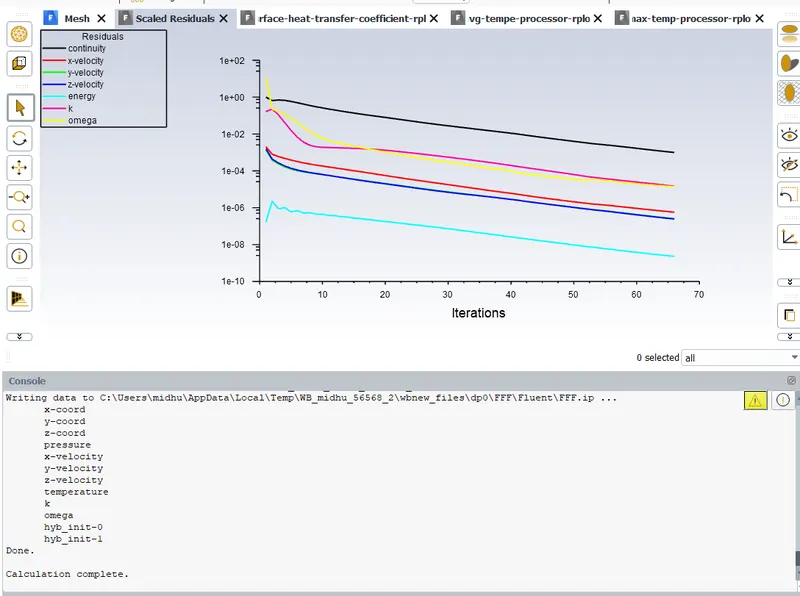
Showing Residuals

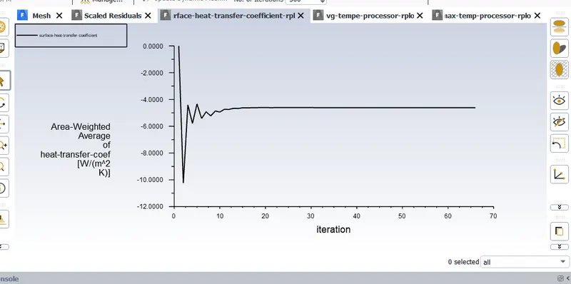
Showing plot of Surface heat transfer coefficient

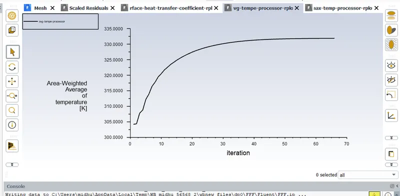
Showing plot of average temperature

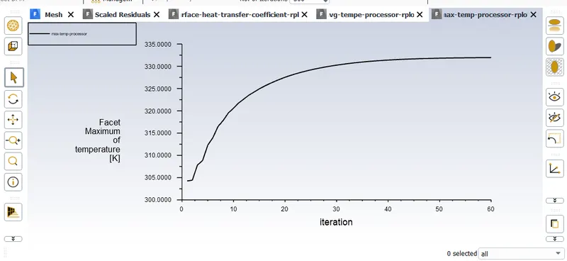
Showing plot of maximum temperature

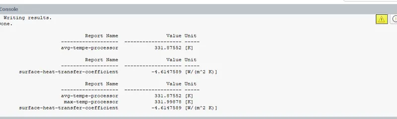
Figure showing the values of Surface heat transfer coefficient,Average temperature and maximum temperture

ie Surface heat transfer coe = -4.614W/m2K(Negative sign is beacuse heat is leaving from the processor)

Average Temperature = 331.8752k

Maximum Temperature = 331.99878K

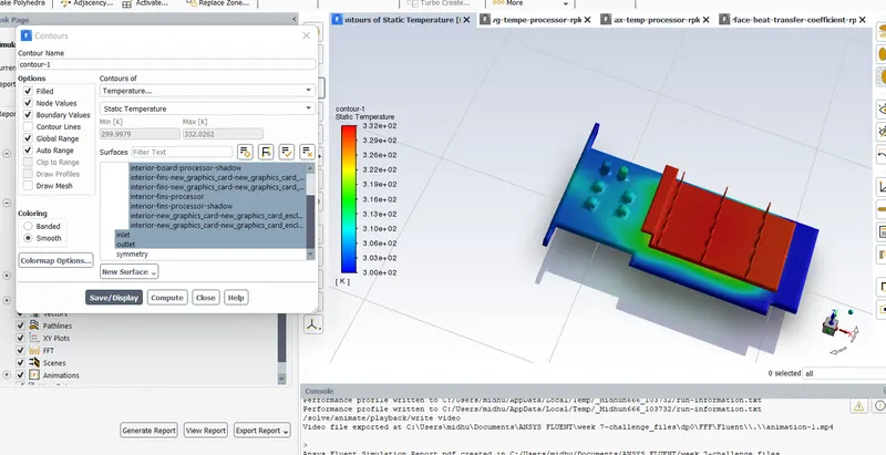
Contour of Temperature Distribution

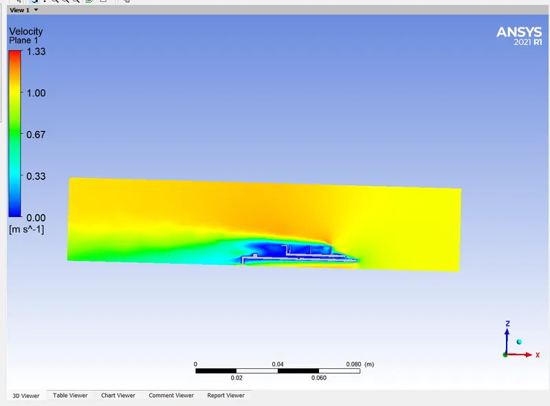
Contour of Velocity Distribution

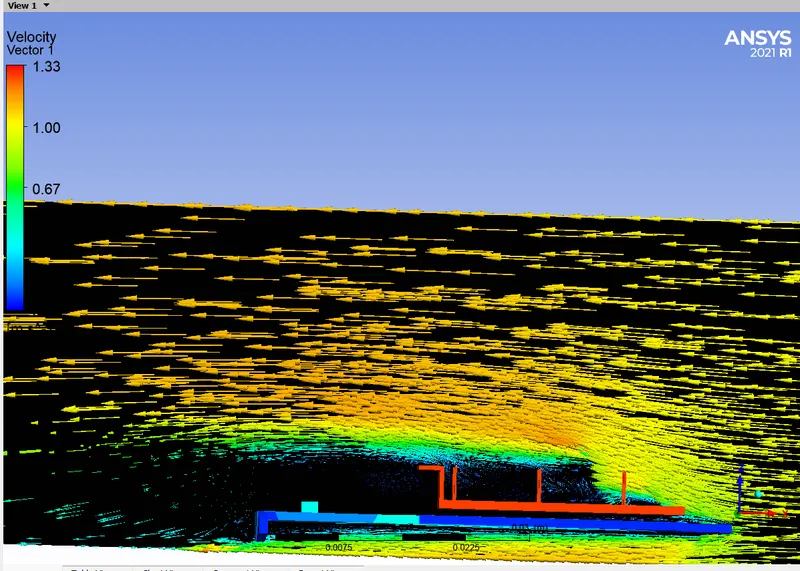
Velocity vector plot

Some wake regions are forming behind the fins due to flow seperation and which due to the obstruction created by the fins in the flow path.

CASE 2: Inlet Velocity 3m/s

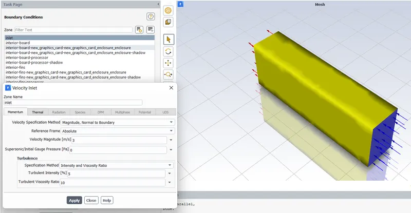
Giving inlet velocity as 3m/s

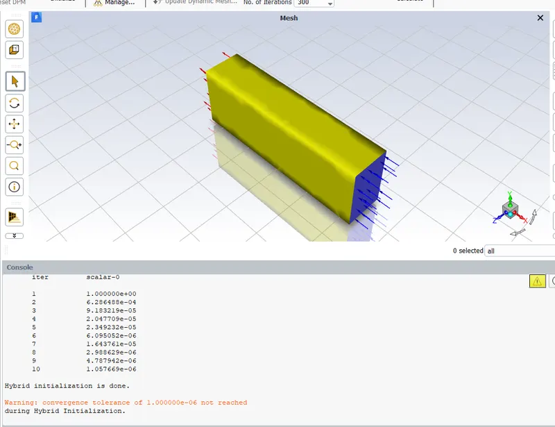
Hybrid Initialization done

RESULTS AND DISCUSSIONS:

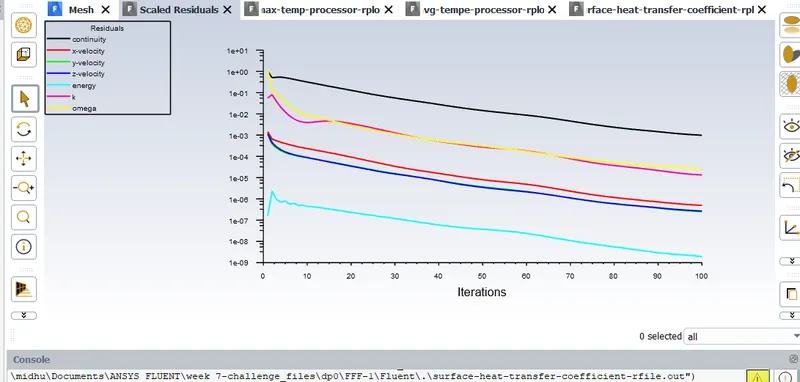
Showing Residuals

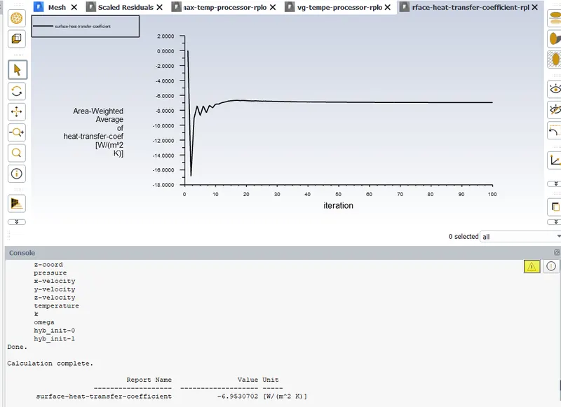
Plot and value of surface heat transfer coefficient.

From this it is clear that surface heat transfer coefficient is -6.95307 W/m2K.

Surface heat tranfer coefficient increases due to the increase in inlet velocity

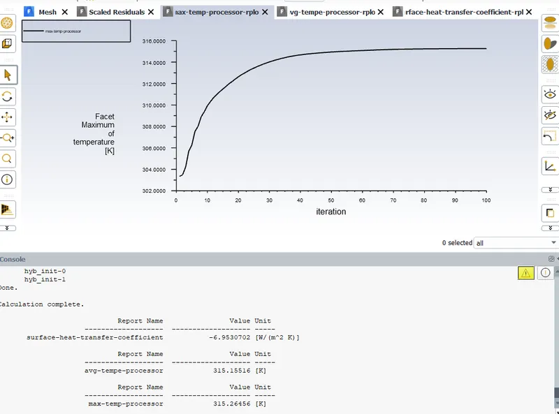
Plot and value of maximum temperature

From this it is clear that maximum temperature is 315.2645K.

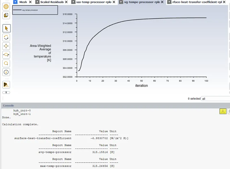
Plot and value of average temperature

From this it is clear that average temperature is 315.1551K.

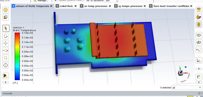
Contour of temperature

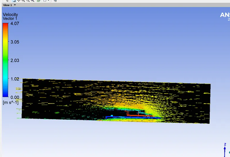
Vector plot of velocity distribution

Generation of wake is more due to increase in velocity

CASE 3: Inlet velocity 5m/s

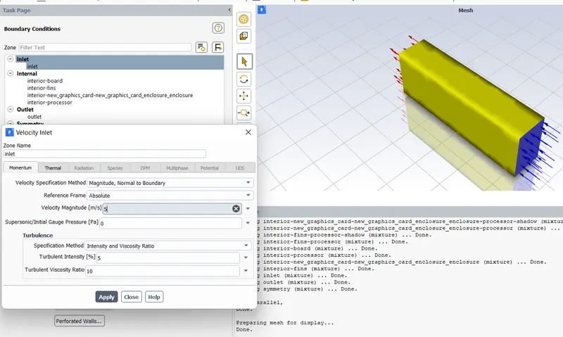
Giving inlet velocity as 5m/s

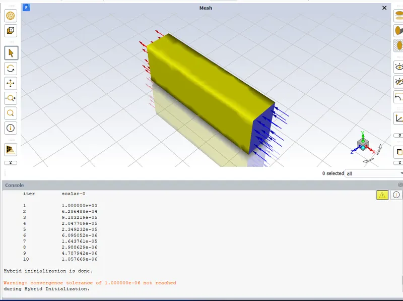
Hybrid Initialization done

RESULTS AND DISCUSSIONS:

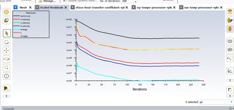
Showing residuals

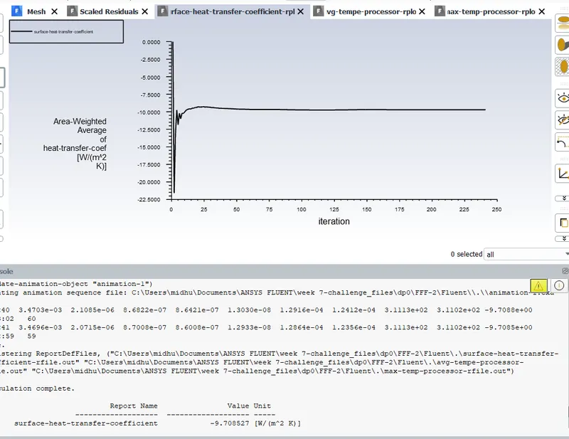
Showing plot and value of surface heat transfer coefficient as -9.708W/m2K

Again value of surface heat transfer coefficient increases ue to increase in inlet velocity

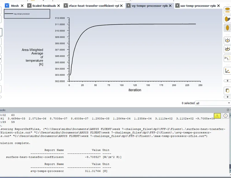
Showing plot and value of avrage temperature as 311.017K

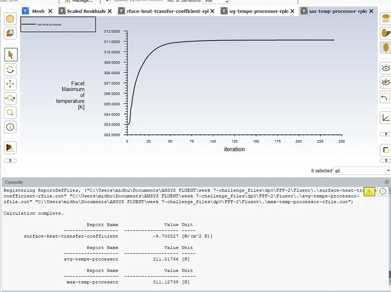
Showing plot and value of avrage temperature as 311.127K

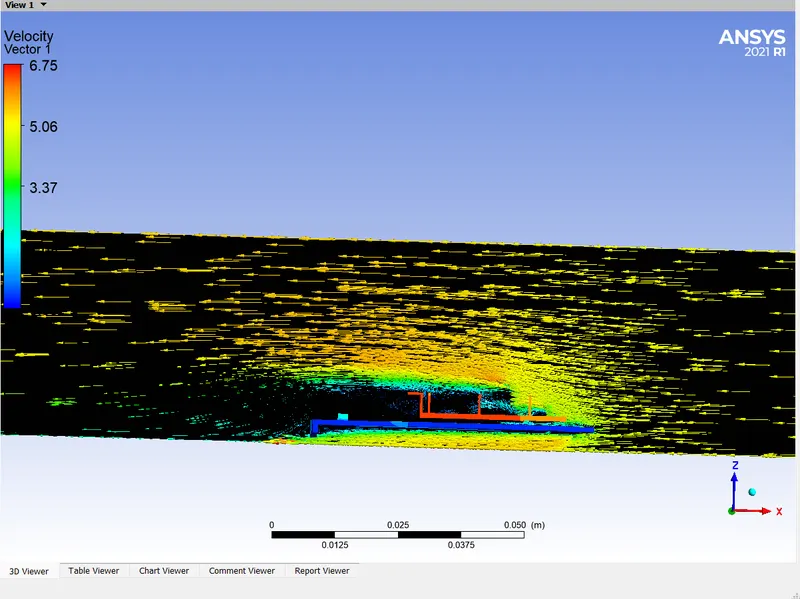
Showing velocity vector plot

MESH INDEPENDANCE STUDY:

Cases	Mesh size	Cell Count	Surface heat transfer coefficient(W/m2K)
(1)	0.0005mm	3,36,762	-4.614
(2)	0.0003mm	6,92,929	-8.8082
(3)	0.0001mm	15,26,385	-8.9145

From this mesh independance study we can understand that, there is no much difference in surface heat transfer coefficient when meash size is 0.0003mm and 0.0001mm.Threfore we can fix the optimum mesh size is 0.0003mm.

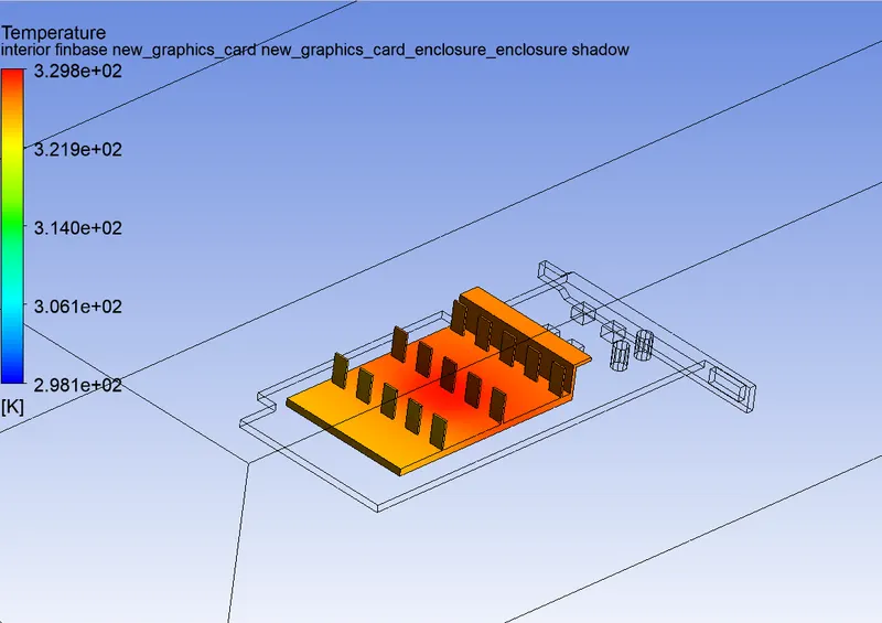
4. Identify potential hotspots on the model.

For identifying the Hotspots we have studied and analyzed several cases for the temperature and HEAT transfer coefficient.

so we know that the most potential Hotspots are around the Fin base and the whole microprocessor.

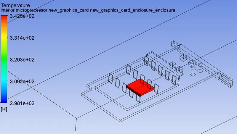
CONCLUSIONS:

(1) When the inlet velocity of flow increasing, the value of surface heat transfer coefficient also increasing and this is beacuse the value of surface heat transfer coefficient is depending on Reynold's number.

(2) The value for each inlet velocity is given in the table as given below:

Inlet Velocity	Surface heat transfer coefficient(W/m2K)
1m/s	-4.614
3m/s	-6.95307
5m/s	-9.708

(3) Mesh independance study done and found the optimum mesh size is as 0.0003mm.

(4) Identified potential hotspots on the model