Week 6 - CHT Analysis on a Graphics card

Aim:- CHT Analysis on a Graphics card

Objective :-

1) steady-state conjugate heat transfer analysis on a model of a graphics card.

2) Select appropriate material for different component in graphics card

3) Simulation has to be on coarse and fine mesh with 3 different velocities starts from 1m/s to 5m/s

4) Find maximum temperature and heat transfer coeffiecient attained by processor

Tools used :-

1) Space claim

2) Ansys mesh

sizing , capture proximity

3) Ansys Fluent

Turbulence model , Material , Cell zone condition, Boundary condition , Initialization , Compute

4) CFD-Post

Contour , plane , velocity vector

Theory :-

Graphics card :-

A graphics card is an extension card which display output images. Graphics card is designed on printed ciruit borad (PCB) having different components which perform different functions, in which there is processing unit which performs necessary computations, consume large amount of power and generates heat , to dissipate the heat generation requires CPU/GPU cooler and fines are designed over graphics card.

Graphics crad are made up of different materials such as poysterene for pcb , silicon for processor. Fins which increase surface area tends to dissipate heat should have material with high thermal conductivity such as aluminium.

This simulation is based on conjugate heat transfer from graphics card and to analyze maximum tmperature reached by processor and heat transfer coefficient.

Procedure:-

1) Preprocesing

grometry

a) Import geometry of Graphics card in space-claim

b) share the topology using share option

* as computational domain is already constructed so no need to construct again

meshing

a) Open Ansys mesh

b) Generate mesh with different mesh size i.e., a coarse mesh and a fine mesh

Type of mesh	Element size	Element number
Coarse mesh	100mm	175777
Fine mesh	60mm	476903

* Here,The selection of element size is based on computaion time and limitation of maximum element number for academic version. And these elements can capture the flow in a nice way.

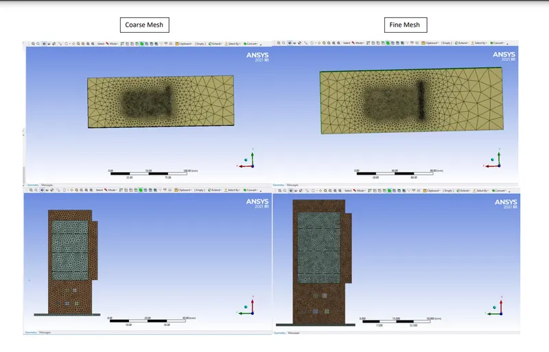
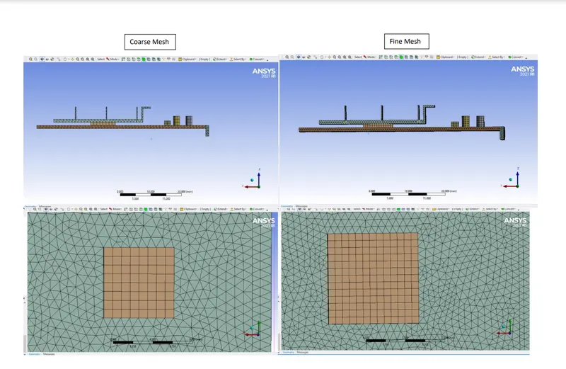
c) Capture proximity is ON , because there are very small components are available on graphics card and that is main concern region for the analysis , so minimum element size should be there.

d) Give name selection as

- Inlet , Outlet , Domain, Processor , Fins , PCB

2) Solving

Solver

a) Open CFD solver,which is Ansys fluent.

b) Here, we are analyzing heat transfer so energy will be ON

c) Flow is incompressible so select pressure based solver and k-epsilon turbulence model

d) Select appropriate materials for different component

Component	Material	Thermal conductivity (W/mK)	Specific heat capacity (J/kg.K)	Density (kg/m^3)
Fin	Aluminium	202.4	871	2719
Processor	Silicon	15.3	703	2330
PCB	Polysterene	0.027	1210	55
Heat transfer fluid	Air	0.0242	1006.43	1.225

e) Here, we are assuming heat capacity of processor be q =2 W

and v=volume= 8*8*1 mm

So, heat generation,qg = q/v

after calculation heat generation is 31250000 W/m^3

so, give this heat generation in energy source of silicon.

f) go to cell zone condition and assign proper solid/ fluid to selected material and give above calculated energy source for processor.

g) Now, In boundary condition, the simulation has to be run on different velocities so let coarse mesh be on 5m/s and fine mesh on 1 ,3 , 5m/s.

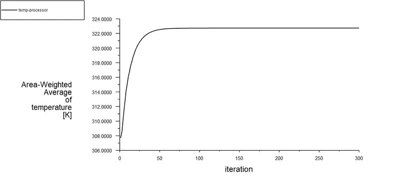
h) Create heat transfer coefficient and processor temperature report definition

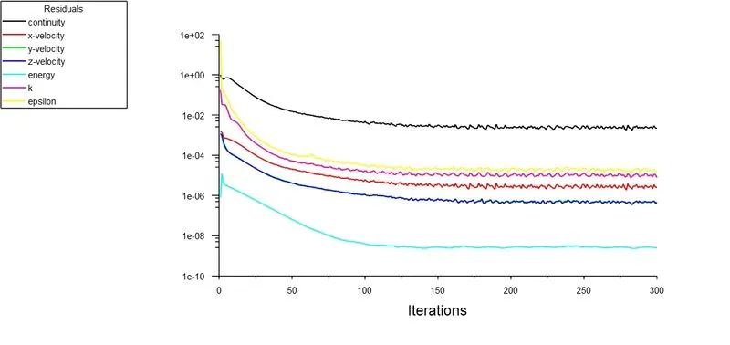
i) Now initialize the simulation and compute for 300 iterations

3) Postprocessing

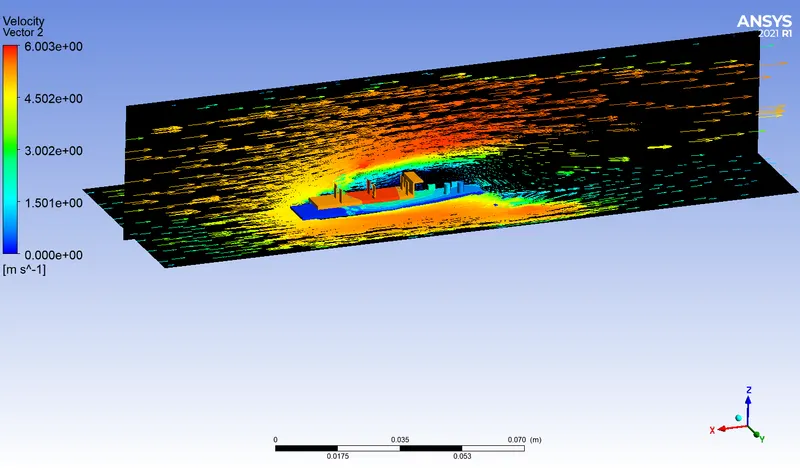
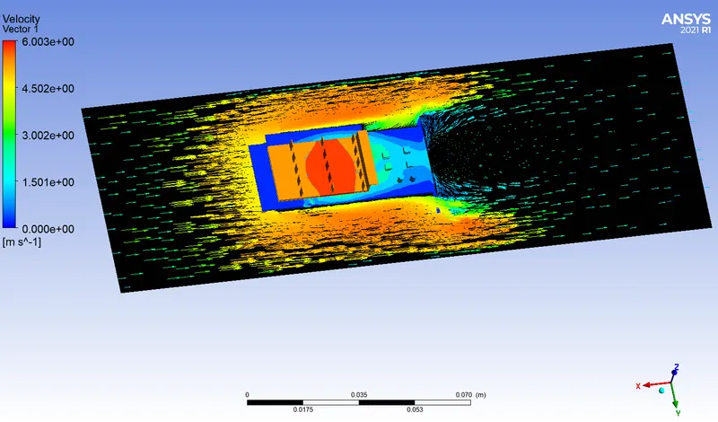
a) Create temperature contour , and velocity vector plot in CFD-Post

Result :-

Type of mesh	Cases	Velocity (m/s)	Max. Processor Temp (K)	Heat transfer coefficient (W/m^2K)
Coarse mesh	Case 1	5	322.73	-15.82
Fine mesh	Case 2	1	352.99	-6.35
	Case 3	3	327.06	-9.81
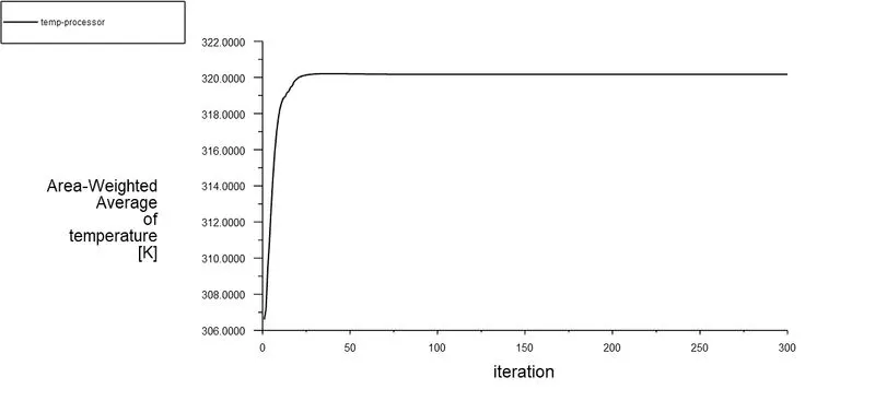
	Case 4	5	320.16	-13.92

Plots & contours :-

Case 1

Residual plot

Processor temperature plot

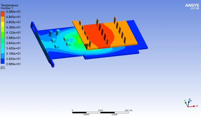
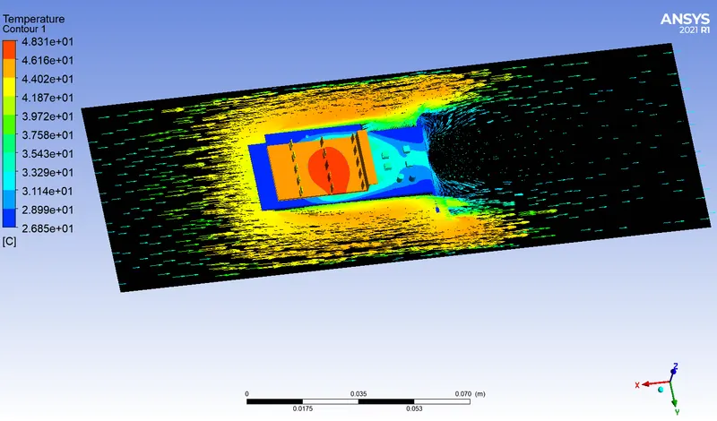
Temperature contour

Velocity vector

Case 2

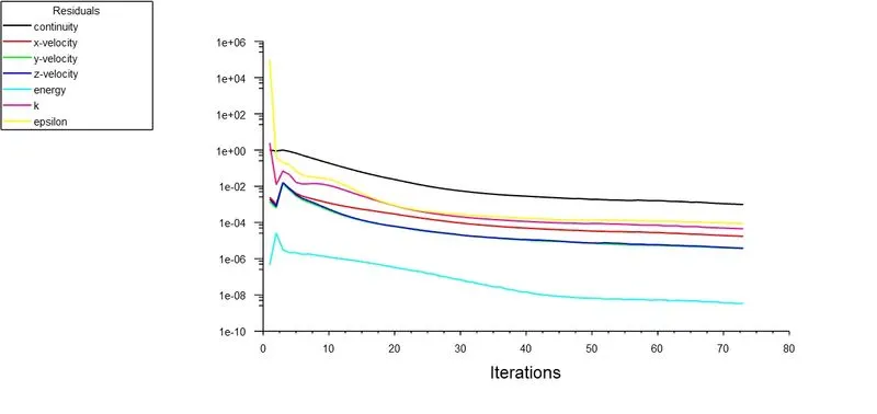
Residual plot

Processor temperature plot

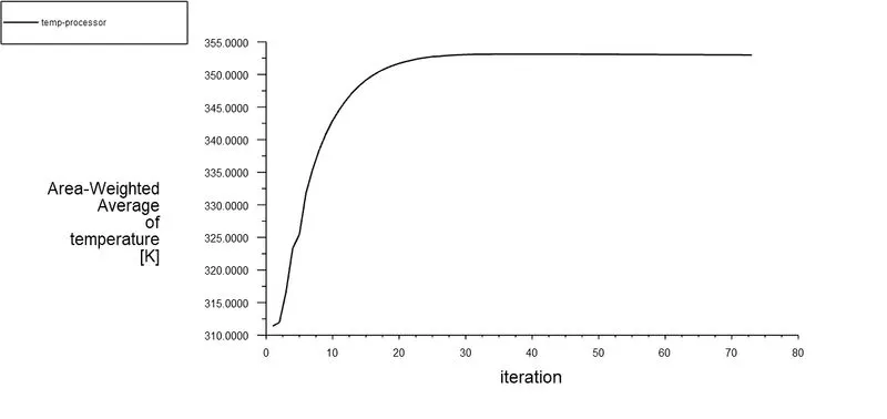
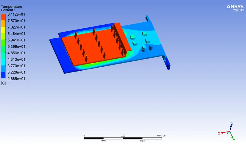
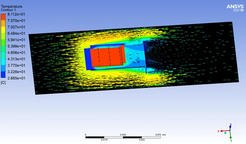
Temperature contour

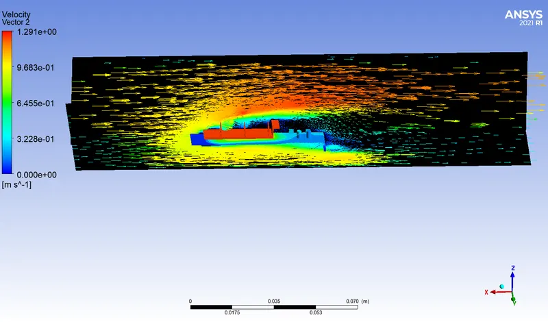
Velocity vector

Case 3

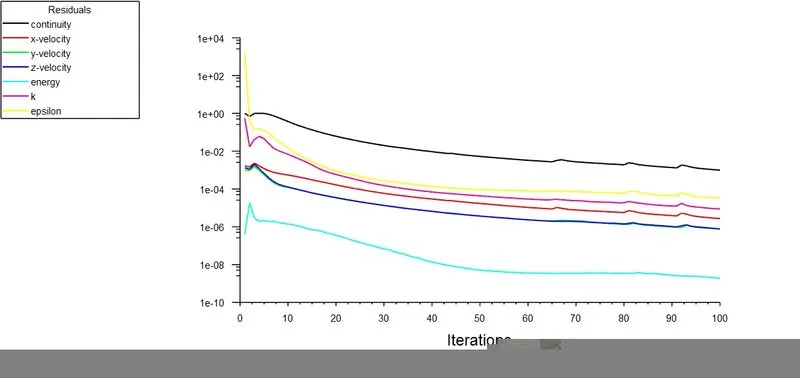
Residual plot

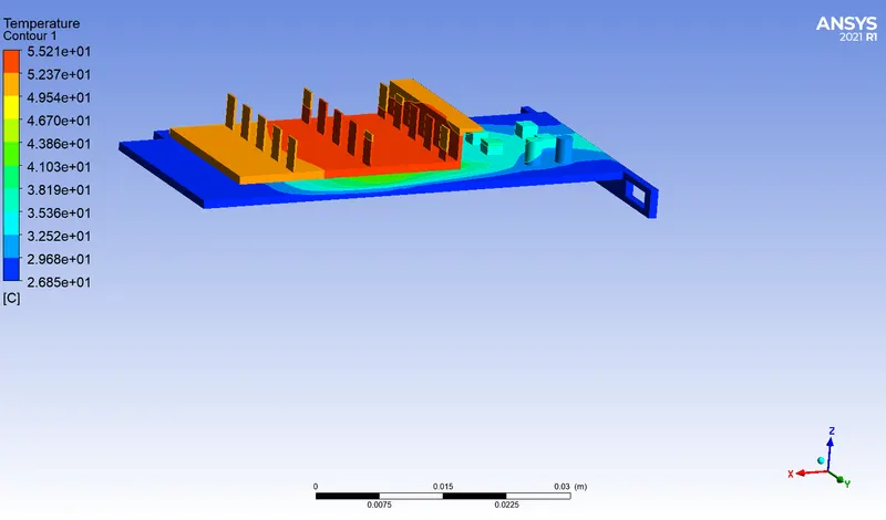
Temperature contour

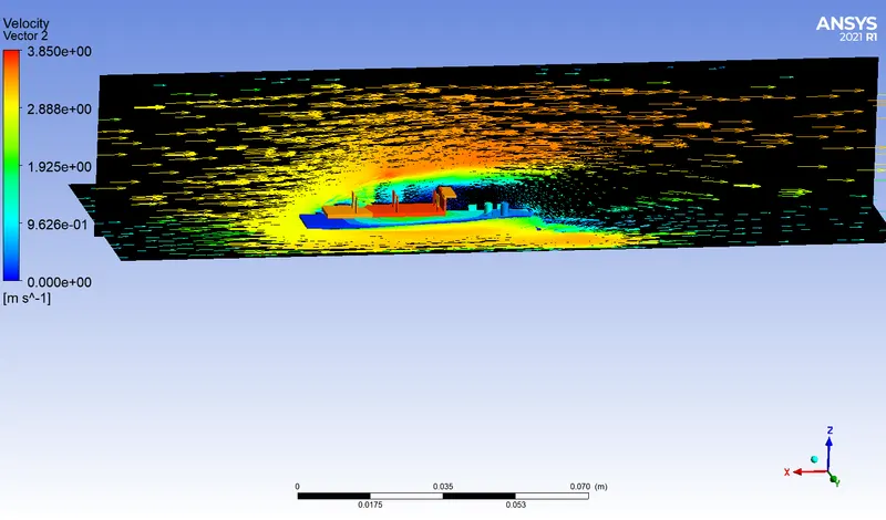
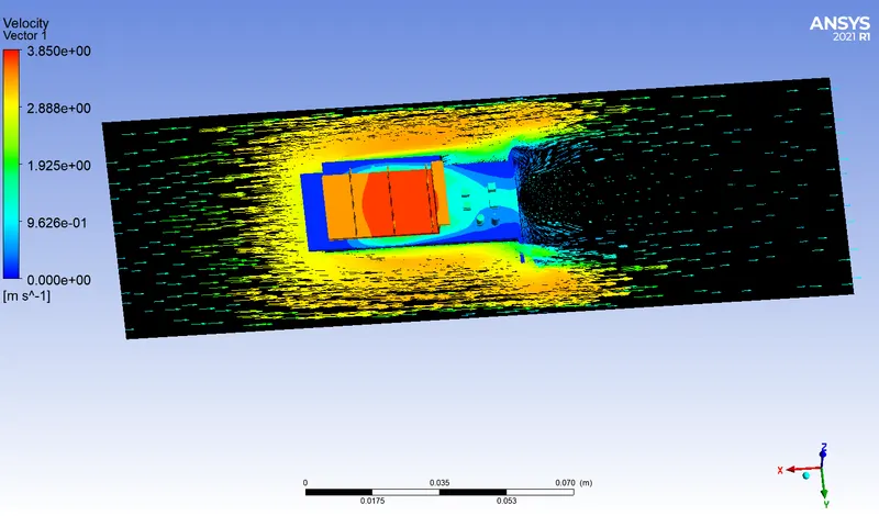
velocity vector

Case 4

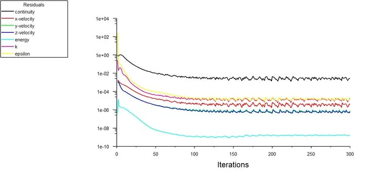
Residual plot

Temperature plot

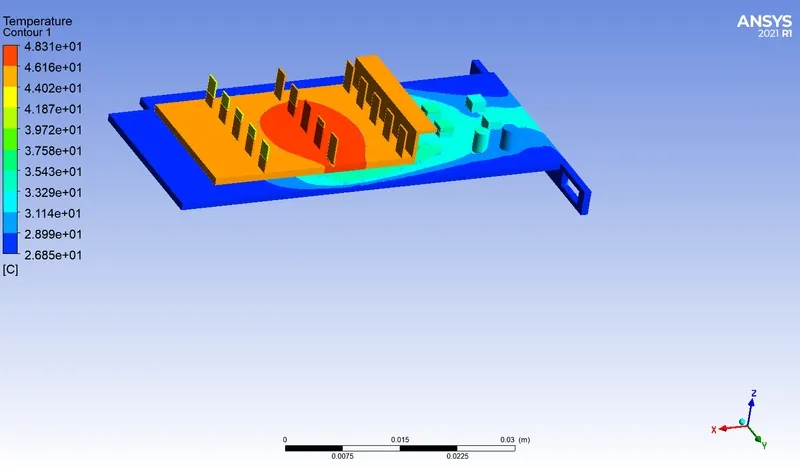
Temperature contour

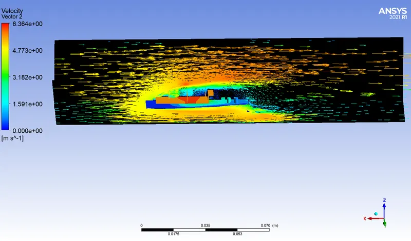
Velocity vector

Conclusion:-

Simulation on graphics card has been done with coarse mesh at 5m/s and fine at different velocity which is 1,3,5 m/s and resultant maximum processor temperature and heat tarnsfer coefficient is found out and is tabulated above.

On comparison with coarse and fine mesh result at 5m/s it has been found that fine mesh have slightly less maximum temperature and heat transfer coefficient than coarse mesh.

Also, it is observed that at different velocity for fine mesh , as velocity is increasing both maximum temperature and heat transfer coefficient is decreasing.

Simulation was run for 300 iteration and Case 2 & 3 converged very early around at 100th iteration.

From temperature contour , it is shown that maximum temperature is at center of Fins i.e., hotspot is at center of fins because it is dissipating heat and processor which is generating heat is just beneath the fins platform.