Week 6 - CHT Analysis on a Graphics card

AIM- Perform steady state heat transfer analysis on Graphic card for different velocity 1m/s , 3 m/s & 5m/s for coarse mesh and fine mesh with all required plots and contnours.

THEORY

Conjugate Heat Transfer

The conjugate heat transfer analysis type allows for the simulation of heat transfer between solid and fluid domains by exchanging thermal energy at the interfaces between them.Typical applications of this analysis type exist as ,But are not limited to simulation of heat exchangers,cooling of electronic equipment and general purpose cooling and heating of systems.Example - HVAC , Heat exchanger ,Tank,Internal combustion engine,Heat sink boiler, Nuclear Reactor etc.

Heat transfer in solids- CONDUCTION is Diffusion of heat due to temperaure gradients in solids. A measure of the amount of conduction for a given gradient is heat conductivity. It is discribed by fourier's Law defining conductive heat flux q, proportional to the temperature gradient.

Heat transfer in fluids- CONVECTION is heat carried away by moving fluid . Which can be due to external influences or forced convection or by buoyancy forces natural convection.

Fluid motion contribute to 3 ways of heat transfer

1. Convective contribution: Depending on the properties of the fluid and its region of flow, Domination of conduction and convection varies.

2. Viscous Effects: Due to fluid dlow , The viscosity creates heat .This effect is often neglected due to its negligible value.But its considered in high velocity cases.

3. Density Effects: When density becomes related to temperature the domain will have different densities at different locations based on themperature distributions.This variation in density can cause the compression which in turn generates the heat.

APPLICTIONS

Conjugate heat transfers methods have become essential part for modeling and investigating natural phenomenon and its engineering aspects. Its usage differ from Aerospace and Nuclear reactors to thermal goods treatment and food processing,From Complex procedures in medicine to atmosphere or thermal interactions in meteorology,Relatively simple units to multistage,nonlinear processes.The applications in specific areas of conjugate heat transfer at periodic boundary conditions and in exchanger ducts are considered two different study cases on their on perspect. As the technology is advancing the use for CHT will become more essential and vast .

STEPS FOR SOLVING

• First we open geometry in spaceclaim and we will find all parts up to date we need no geometry clean up and just share the topology if not shared. otherwis data may not be appropriate.
• Then we open geometry in mesh where first we solve for coarse mesh (10mm for enclosure and 2mm for graphic card) and for Finer mesh(3mm for enclosure and 0.65 mm for graphic card bodies)
• In meshing we give outer enclosure different size and use sizing method for changing mesh size for inner bodies.
• We then give names to parts via name selction inlet, outlet, processor, fins, PCB & walls
• After mesh we open the solver where will use Energy mode on with k-epsillon solver ,Steady based and pressure solver as settings to solve the both cases.
• After assigning method we use create material where we already have aluminium,& air But we need to create more material as processor is basicaly made of silicon and PCB(motherboard ) is made of FR-4(laminated glass epoxy materials) .
• We create material by copying alluminium and changing name so we can giver user defined data and we change data using data book or internet.
• After we open cell zone and assign material to proper part Fins is made of solid, Processor of silicon and PCB of FR-4. all being solid type just one fluid air that being passed as cooling method .
• Then we give energy source for processor for 2Watts which is equal to 31250000 W/m^3.
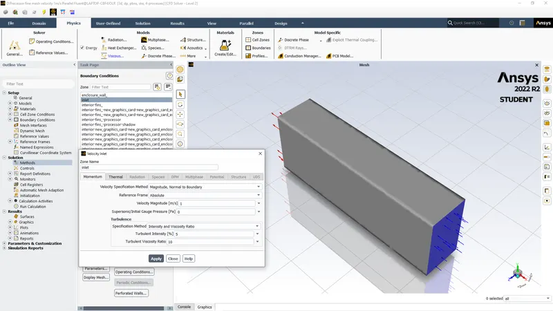
• After we open boundary condition and give velocity of 1,3,5 m/s at inlet for each case.
• We initialize the model and Create graph report for temperature at processor and Heat transfer coefficient at Graphic card surface.
• We the run for 300 iterations.

SOLVING WITH SNIPPETS

CASE-I COARSE MESH( MESH SIZE OF ENCLOSURE IS 10MM AND FINS,PCB & PROCESSOR IS 3MM) for 1m/s, 3m/s & 5m/s velocity at inlet

Geometry

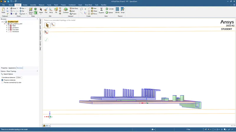
We open geometry in spaceclaim and we find all models updated just we need to share topology.

Parts

Processor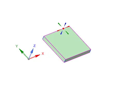

Fins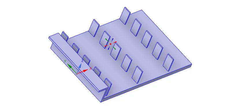

PCB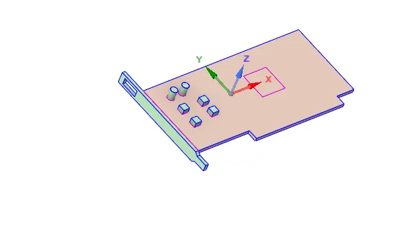

Enclosure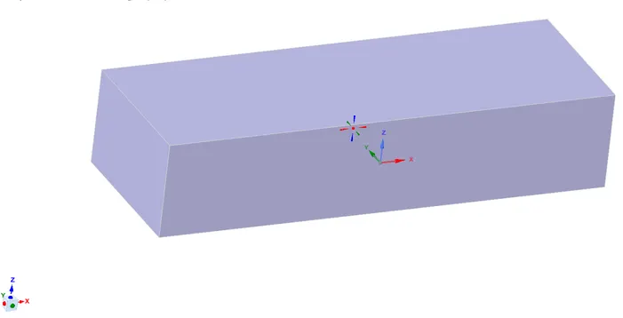

Then we just use share topology

Meshing

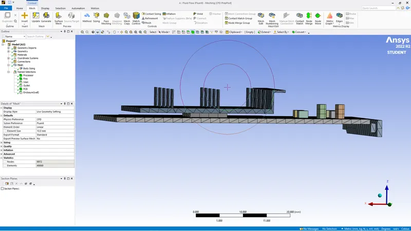
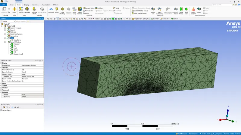
For course mesh we give initial and default data for 10mm for enclosure and 3mm for fins,PCB and processor

We give default mesh then we use sizing method for selected bodies as mentioned for 3mm size

Then we give name selctions to parts

INLET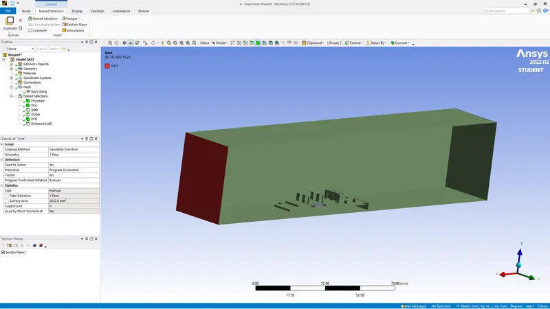

OUTLET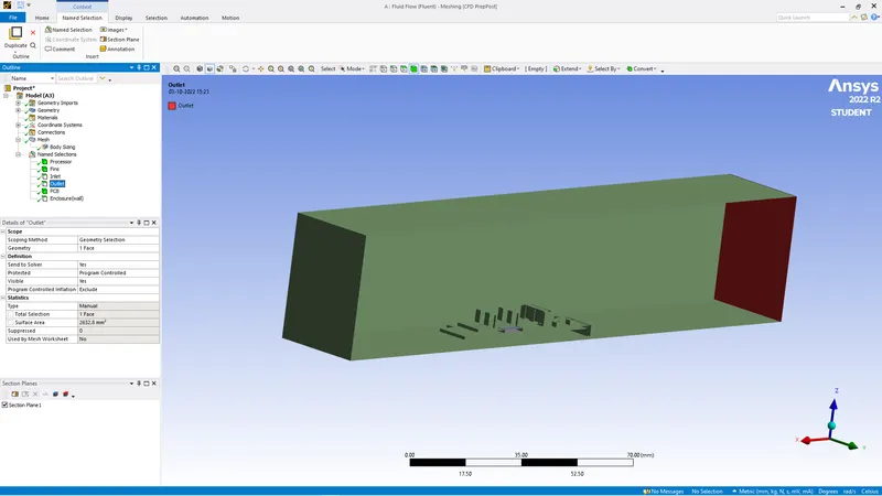

WALLS(ENCLOSURE)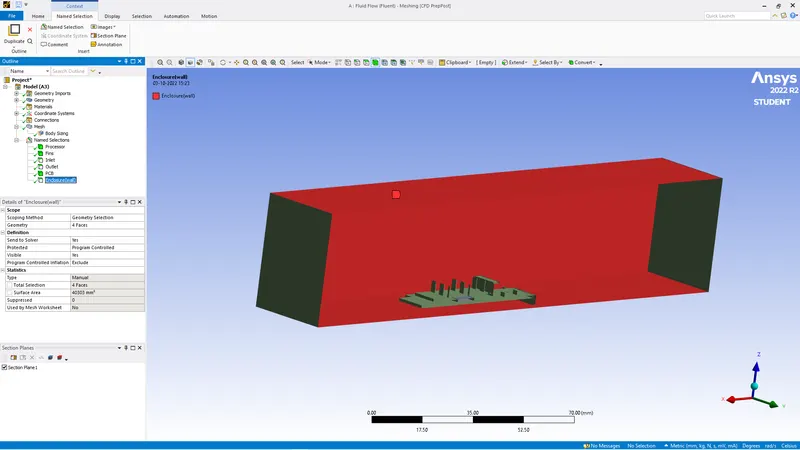

PCB

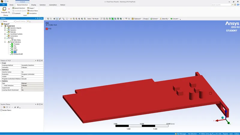
PROCESSOR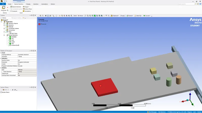

FINS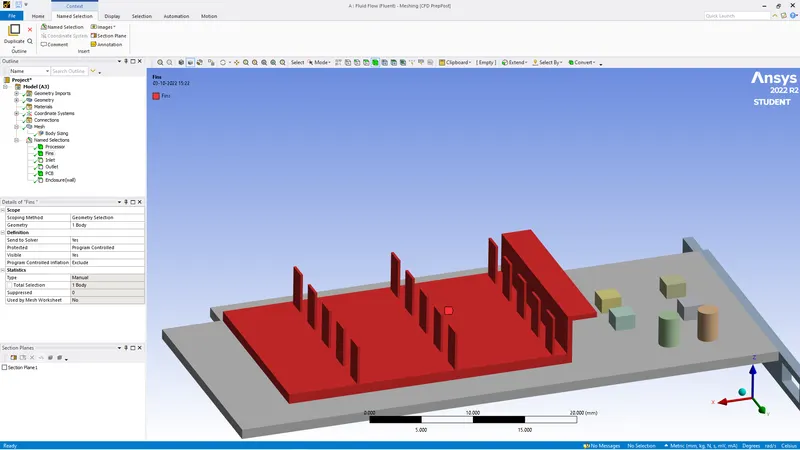

Solver

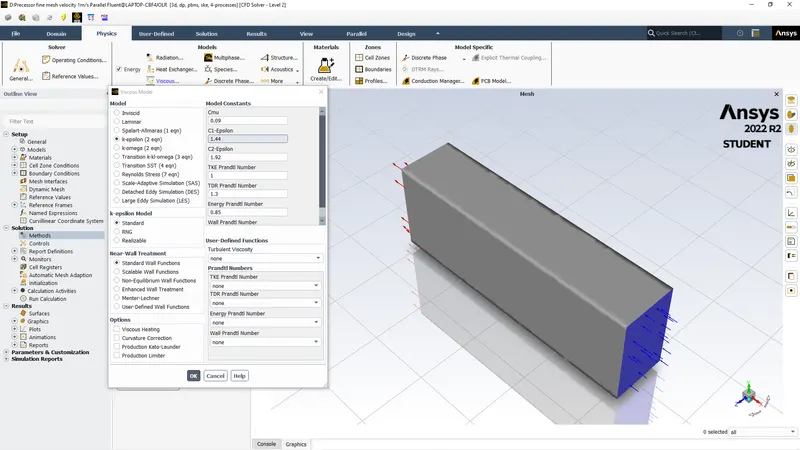
We open model in solve ANSYS FLUENT SOLVER where we use Pressure based model, steady state with energy eqn on and k-epsillon solution solver

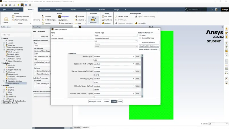
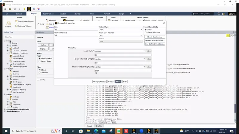
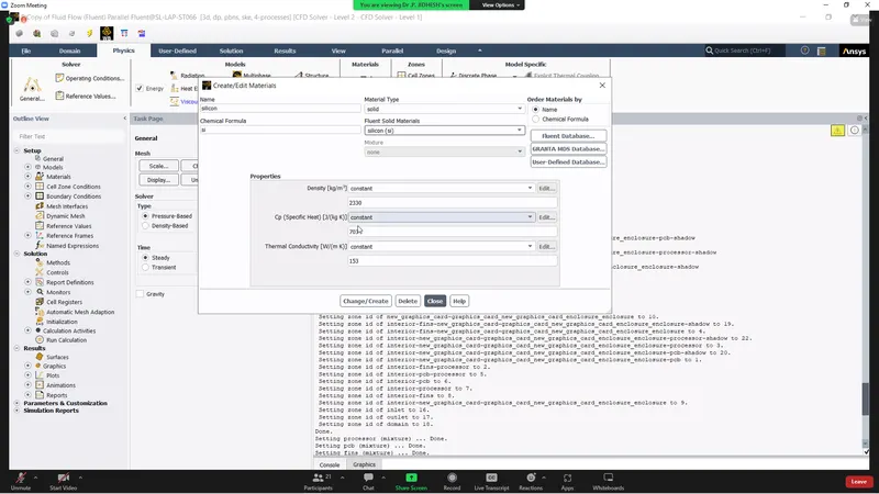
Then we assign data by copying the material of solid and assigning data as follows

MATERIAL	THERMAL CONDUCTIVITY(K)	DENSITY(RHO)	SPECIFIC HEAT (cp)
SILICON	230	2330	710
FR-4	0.294	1850	1150
ALLUMINIUM	2024	2719	871
AIR	0.0242	1.225	1006.43

We go to cell zone and apply these material to the parts Fins is alluminium made, PCB is FR-4 which is glass fibre Processor is made of silicon and velocity medium of fluid is air for cooling purpose.

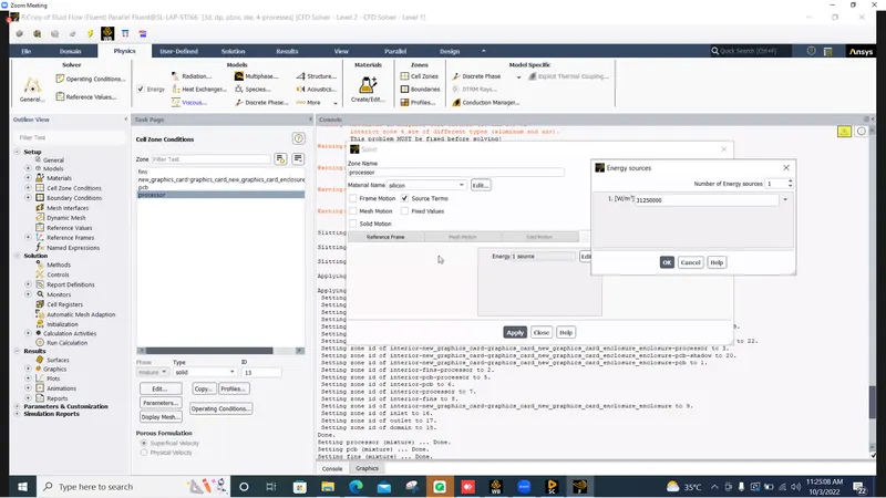
After this we provide the energy source for processor for 2 Watts Then h=3165000 w/m^3

This comes as h= Energy / volume

Where volume = 8x 8 x1 which is size of processor but it is in mm

so h= 2/64 X 10^9 for converting mm into metre so we get 31650000.

After giving energy source we give inlet velocity 1m/sec then 3m/s & 5m/s

Then we initialize and create report for Heat transfer coeffiecient and temperature increase for processor for each velocity case the result is differnt scenerios is as follows.

RESULT FOR VELOCITY = 1M/S

Residual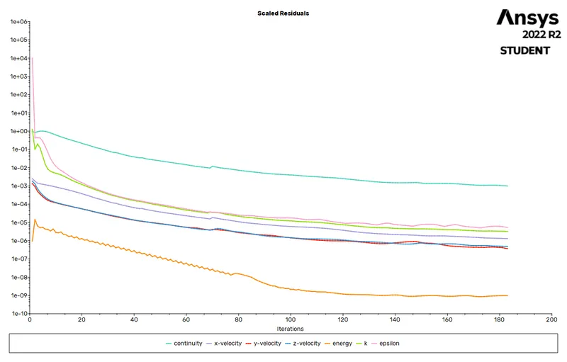

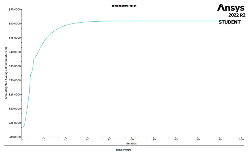
Temperature plot

Heat Transfer coefficient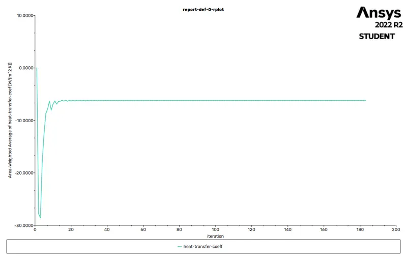

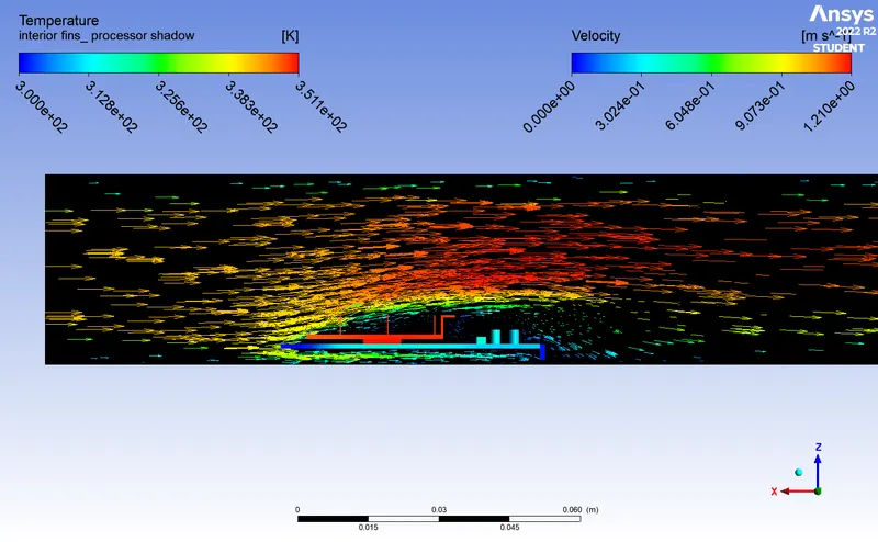
Velocity vector

Temperature contours for different parts and body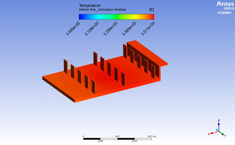

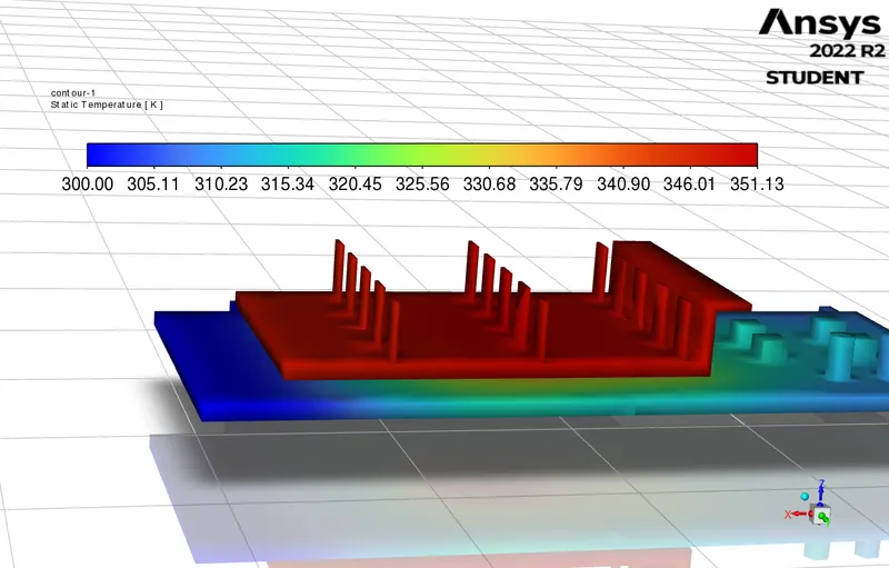
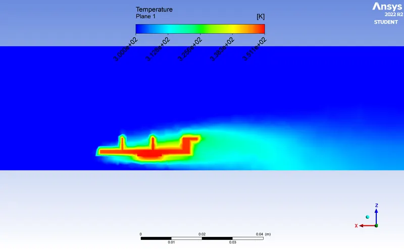
Due to coars mesh size the result is not efficient we can see in plane contour that body imprint is not proper.

Avg Temperature = 350.1 K , Heat transfer coeff.= -6.213 W/m^3

no of elements = approx 162000

RESULT FOR VELOCITY = 3M/s

Residual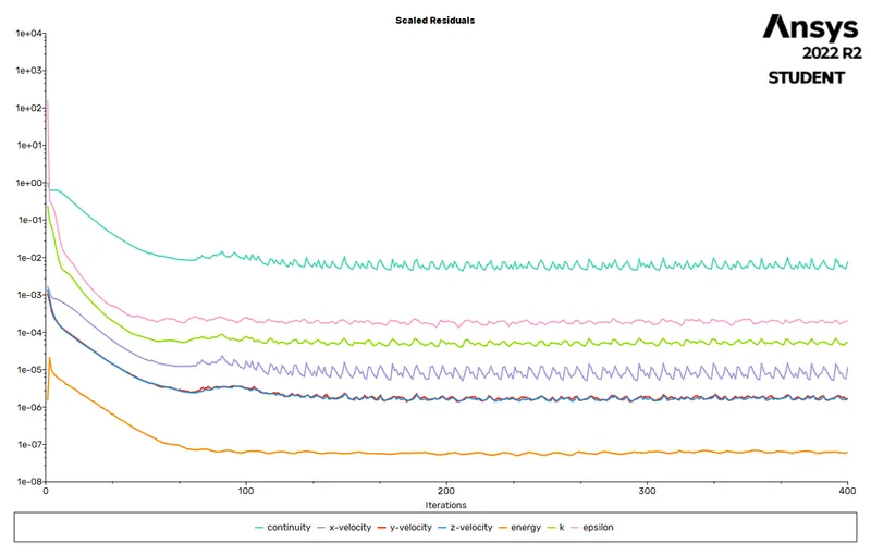

Avg Temperature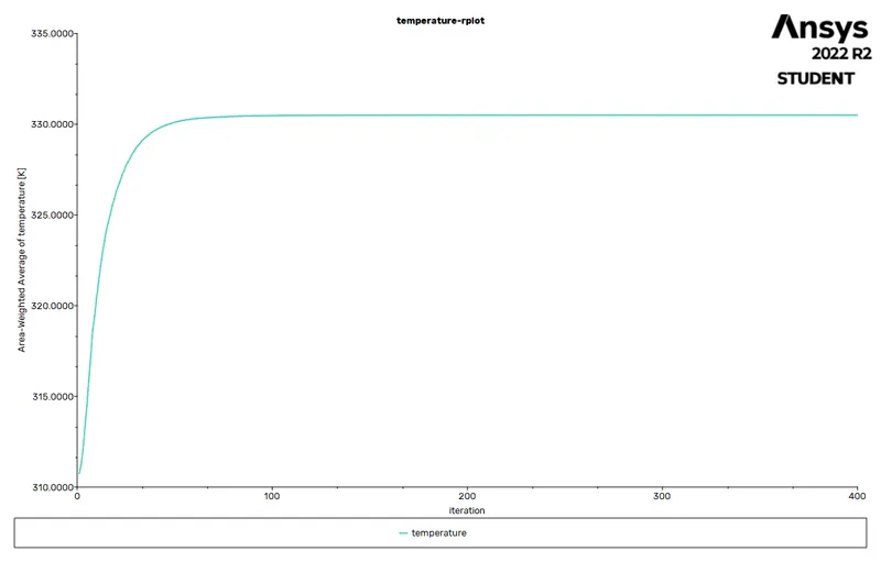

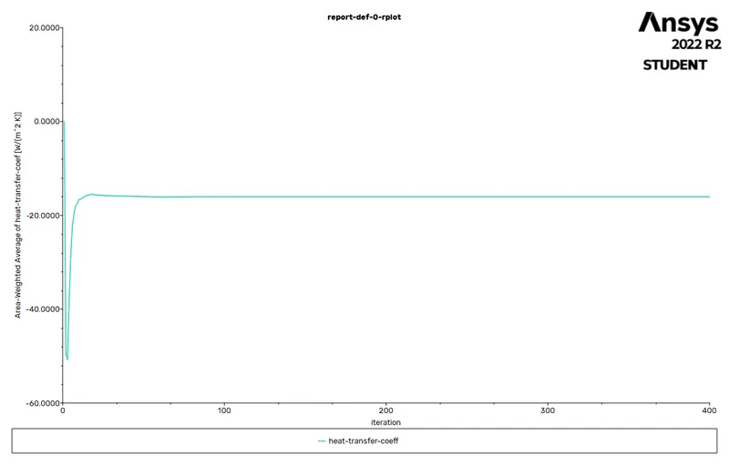
Heat Transfer coefficient

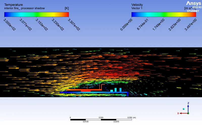
Velocity vector & graph

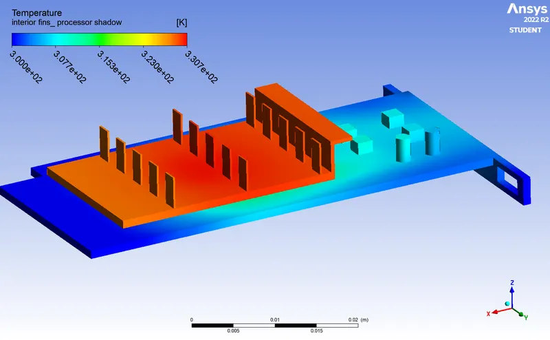
Temperature contour & graph for parts and body

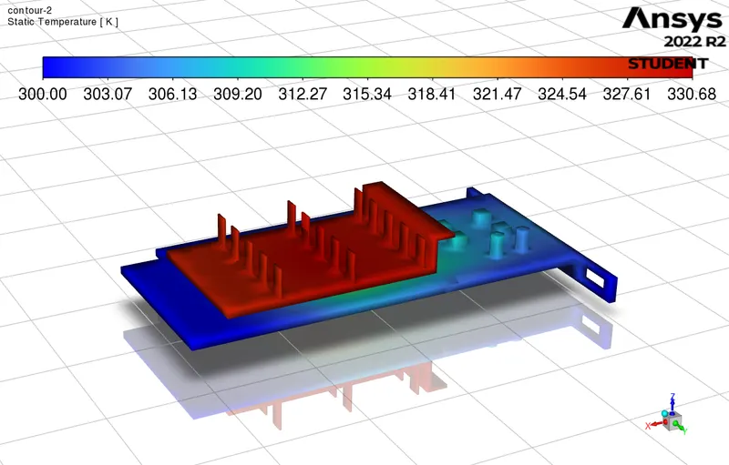
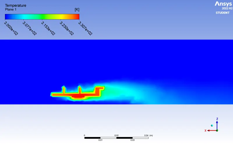
Avg. Temperature = 330.05K & heat transfer coeff= -16.034

RESULT FOR VELOCITY = 5M/S

Residual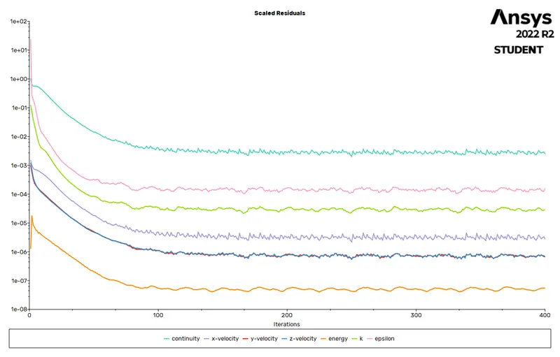

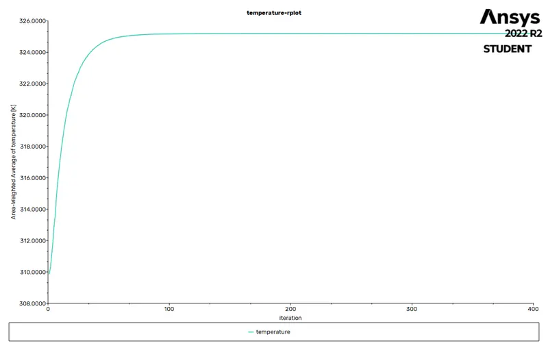
Temperature plot

Heat Transfer coefficent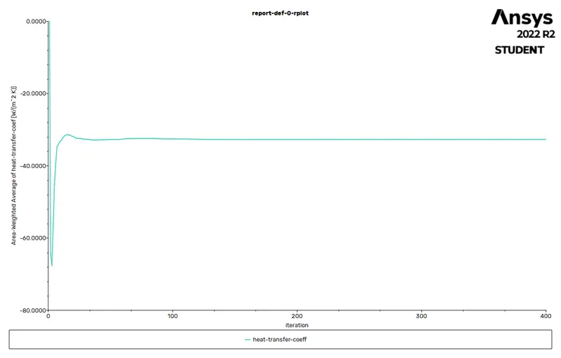

Velocity Vecotor and graph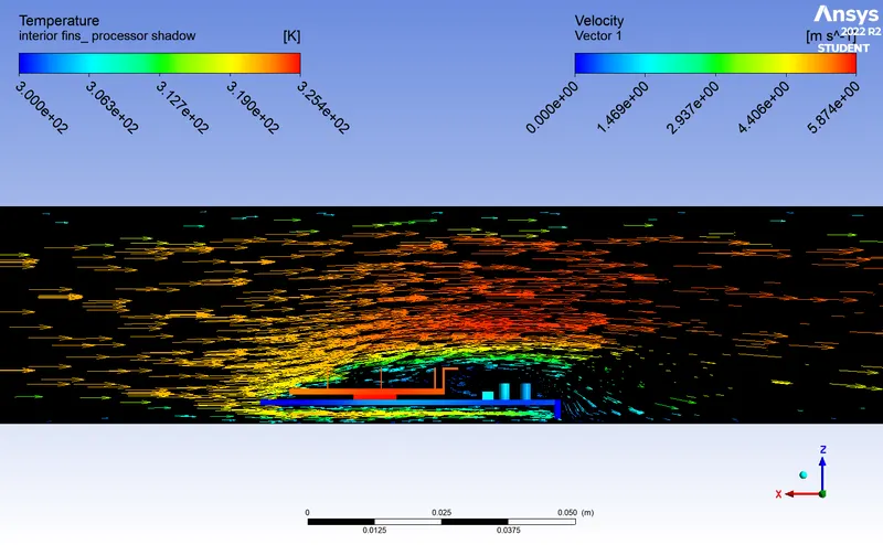

Temperature contour and hotspot for parts and body

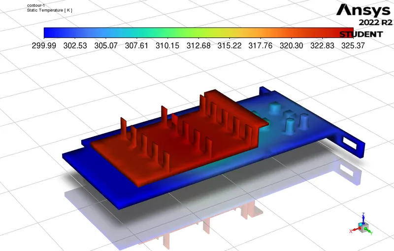
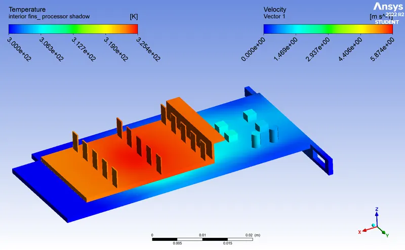
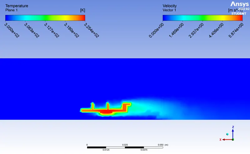
Avg Temperature= 325.19 K & heat transfer coeffcient = -32.72 W/m^3

CASE-II FINE MESH ( ENCLOSURE SIZE= 3MM & FINS, PCB AND PROCESSOR = 0.65MM) FOR VELOCITY 1M/S, 3M/S & 5M/S

All Processes are same just we change mesh size for the body sizing and enclosure sizing

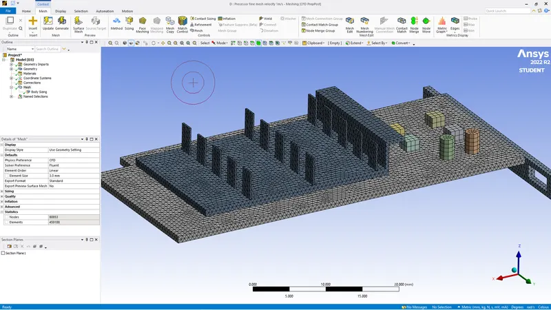
Then we run for same solver method and for different velocities the results are

RESULT FOR VELOCITY = 1M/S

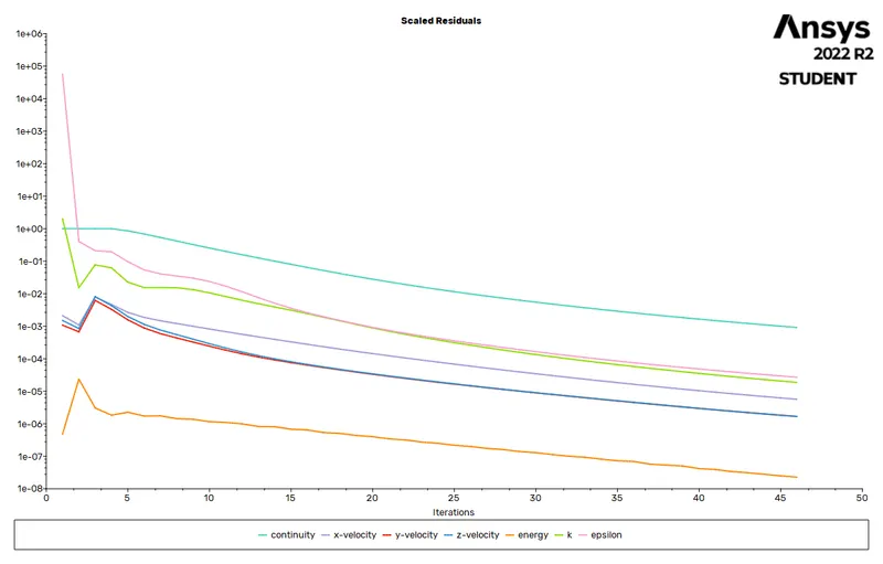
Residual

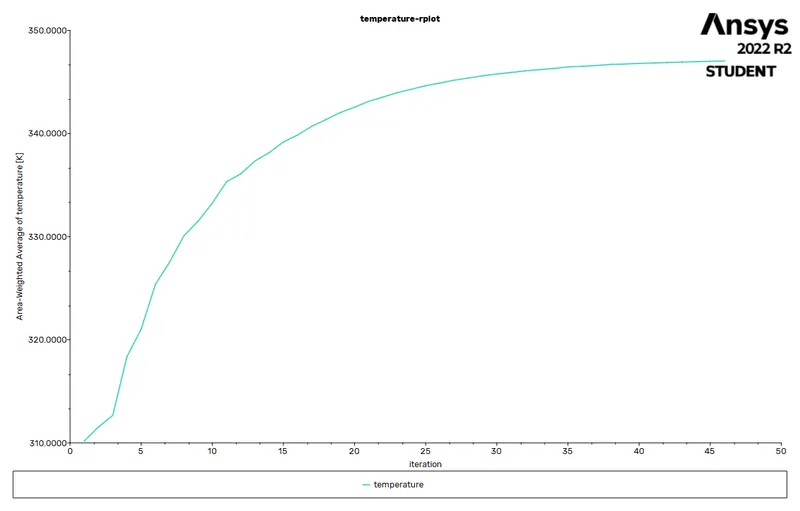
Temperature

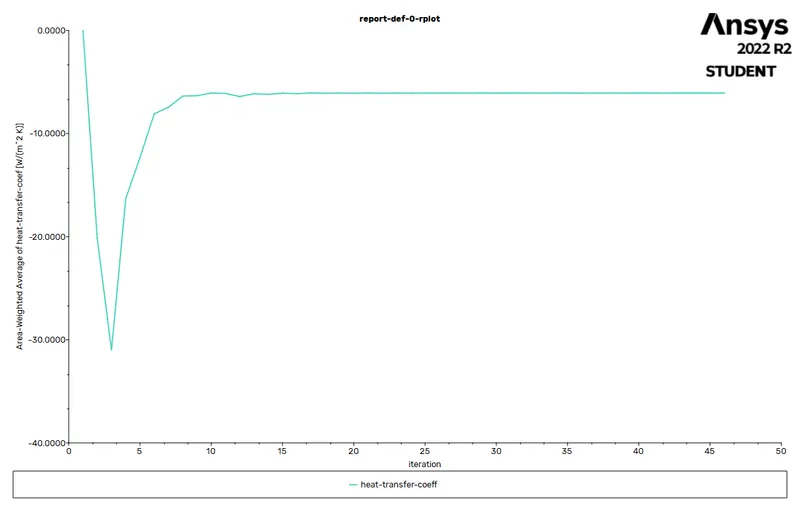
Heat transfer coefficient

Velocity vector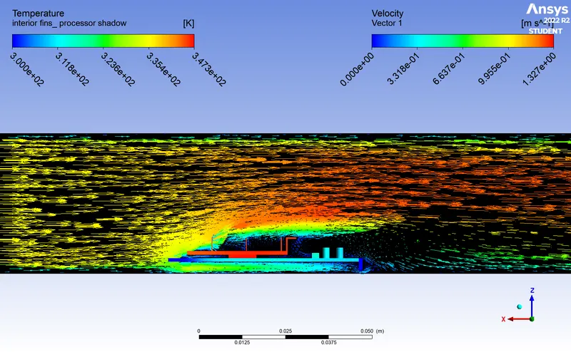

Temperature contours and hotspots on body

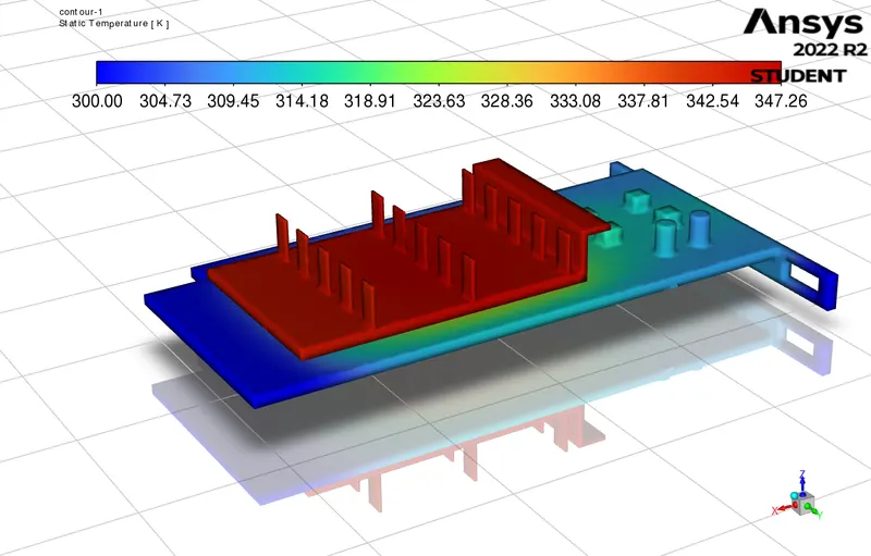
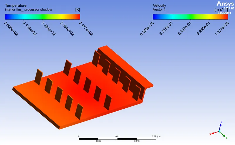
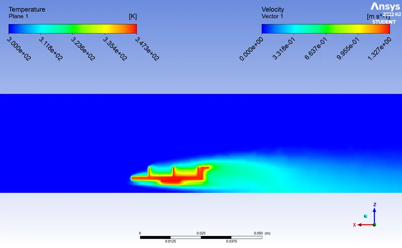
Avg temperature= 347.04K & Heat ransfer coefficient = -6.07 W/m^3

RESULT FOR VELOCITY = 3M/S

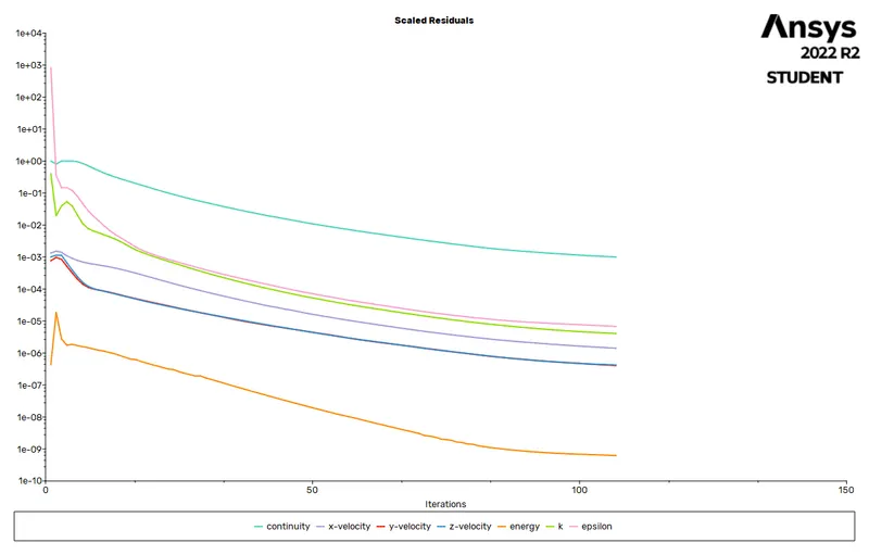
Residual

Temperature plot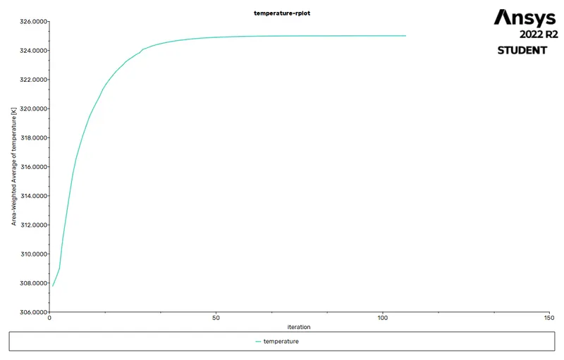

Heat transfer coefficient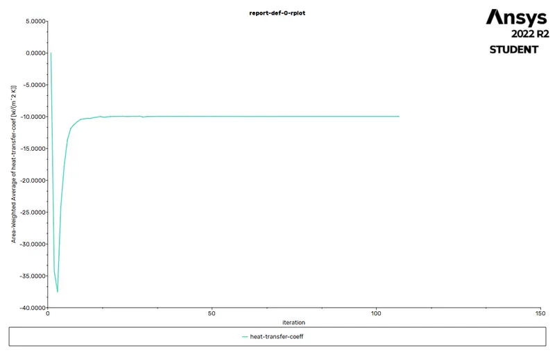

VElocity vector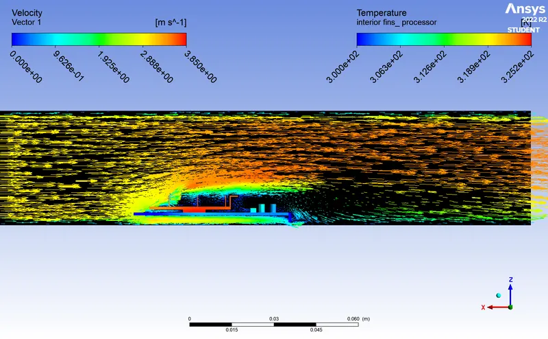

Temperature contours and hotspots for body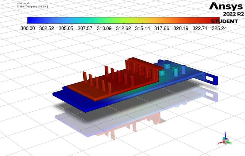

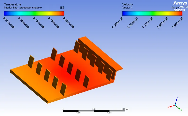
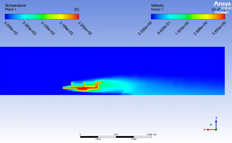
AVg Temperature= 325.5 K & heat transfer coeff= -9.967 W/m^3

RESULT FOR VELOCITY = 5M/S

Residual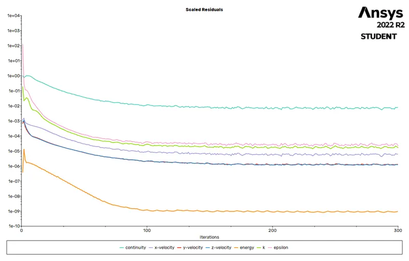

Temperature plot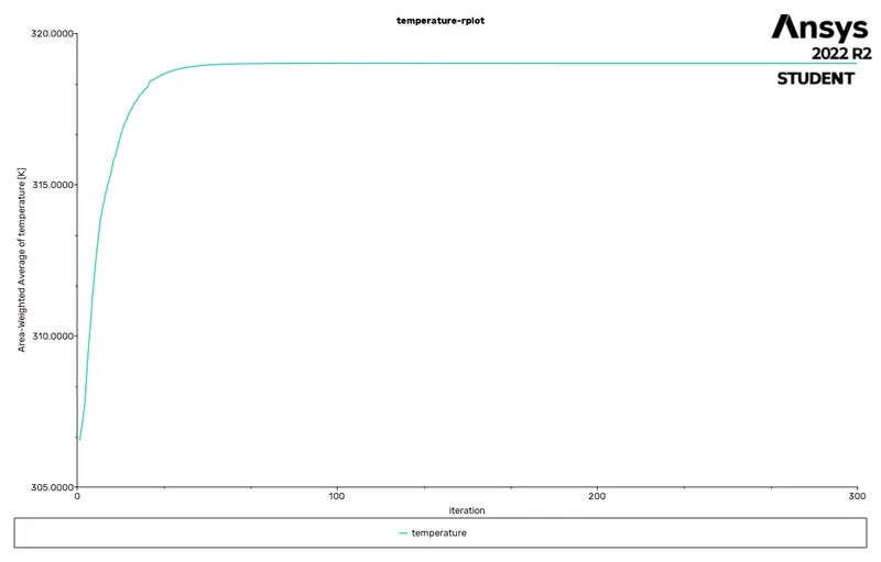

Surface Heat transfer coefficient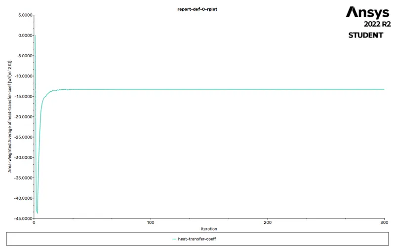

Velocity vector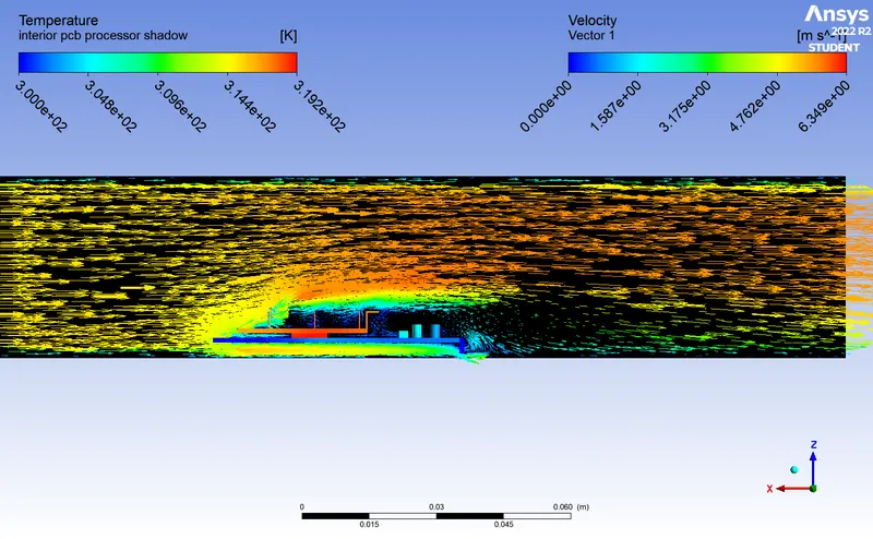

Temperature contour and hotspots on body

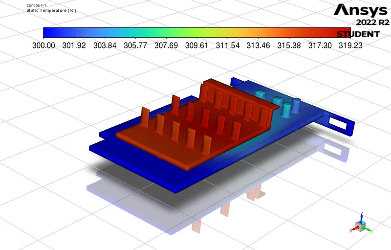
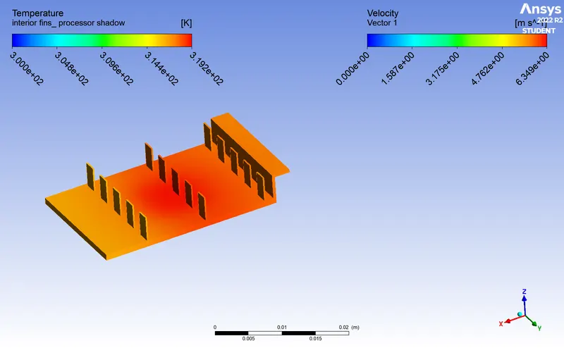
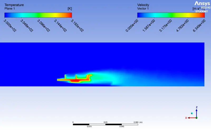
Avg Temperature= 319.01K & heat transfer coeff = -13.251 W/m^3

Conclusion of results

	Coarse mesh velocity 1m/s	Fine mesh velocity 1m/s	Coarse mesh velocity 3m/s	Fine mesh velocity 3m/s	Coarse mesh velocity 5m/s	Fine mesh velocity 5m/s
Avg Temperature	350.1 K	347.03	330.05K	325.05K	325.19 K	319.01 K
Heat transfer coeff.	-6.213	-6.07	-16.034	-9.967	-32.72	-13.251
No. of elements	1,62,000	4,59,188	1,62,000	4,59,188	1,62,000	4,59,188
Convergence after Iterations	183	46	256	107	400	300

We can see that when we deacrease size exponentiay the quality fo Contours and Tempeature hotspots are refined , We find exact values for the Temperatures and the Heat transfer coefficients as we decrease mesh size.
Also the solutions get converge faster this happens as size of element decreases the error in next step calculation decreases due to which convergence happens faster.

Conclusions

• Higher the velocity in region means higher reynolds number. That's why heat transfer coeffient is higher for high velocity case.Which also means maximum amount of heat transfer is taking place in that place.
• HEat transfer coefficient is a function of properties of fluid at film temperature, temperature difference ,coefficient of temperature hence mesh resolution near walls have higher impact of results.
• In any model meshis important parameter as we can see finer the mesh the accuracy of result increases even though time for solving may increase too.
• We can see differnt hotspots happening behind processor which was due to wake region behind the processor area and more heating of processor and coolig around area.