Week 6 - CHT Analysis on a Graphics card

AIM

Steady-state conjugate heat transfer analysis on the exhaust port.

EXPLANATION

CHT Analysis

The conjugate heat transfer (CHT) analysis allows the simulation of heat transfer between solid and fluid domains by exchanging thermal energy at the interfaces between them. In solids, conduction often dominates whereas, in fluids, convection usually dominates.

Typical applications of this analysis type exist as, but are not limited to, the simulation of heat exchangers, cooling of electronic equipment, and general-purpose cooling and heating systems. CHT analysis can accurately predict heat transfer by simultaneously solving all the relevant solid and flow field heat transfer processes, for example, conduction through solids, free and forced convection in the gasses/fluids and thermal radiation.

The CHT approach has an advantage over others such as FE thermal analysis in the wall heat transfer coefficients and their local variations on surfaces are directly calculated within the model rather than based on simplified empirical calculations. The CHT approach, therefore, has benefits for those applications where a transfer is either non-uniform or difficult to calculate empirically.

CASE

CHT analysis on the model of the exhaust port

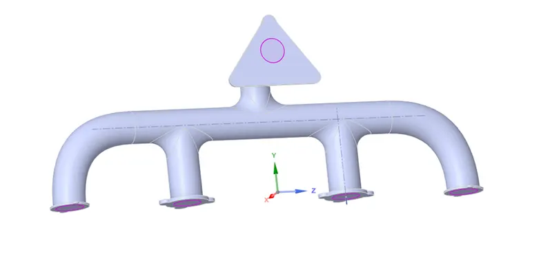
Here an inline four-cylinder engine exhaust manifold is considered, where the conjugate heat transfer is analyzed to find the optimum heat transfer coefficient. Fluid volume is extracted from the port and considered the fluid domain where the air (fluid) enters.

PROCEDURE TO SET UP THE CASE

SpaceClaim

• Geometry preparation in SpaceClaim.
• Removal of extra edges.
• Fluid volume is extracted.
• Final geometry containing both the fluid volume and solid volume generated.
• Enable share topology to ensure the smooth flow of heat from the fluid to the solid.

SpaceClaim can share topology (face, edge, and vertex connections) between touching or intersecting bodies and surfaces in designs that are transferred to ANSYS. Shared topology is the only way to achieve a conformal mesh where bodies meet and is the only way to be certain that the intersection of bodies has meshed perfectly. Shared topology also applies to volume and surface bodies that are completely inside of the other volume or surface bodies. This situation is common in analyses involving fluid flow.

Mesh

• Name surfaces according to respective boundary conditions are created.
• Generate mesh with inflation layer maintaining the y+ value according to the turbulence model.

Name selection – Inflation Layer

Inflation option – First Layer Thickness

First layer height – 0.06 mm

Maximum layers – 10

Growth rate – 1.2

• Body sizing for the inside fluid domain to make the mesh finer.

Body Sizing

Definition – Fluid volume

Type – Element size

Element size – 21 mm

• Statistics

Nodes 190639

Elements 478629

Mesh (y-z plane)

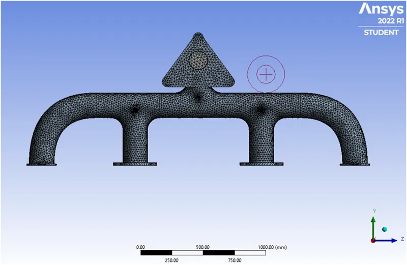
Mesh showing inlets

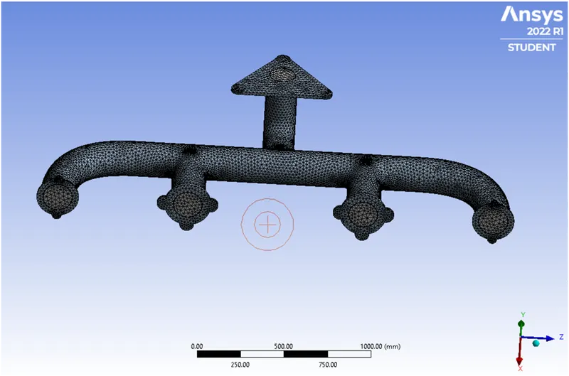
Inlets with Inflation layer

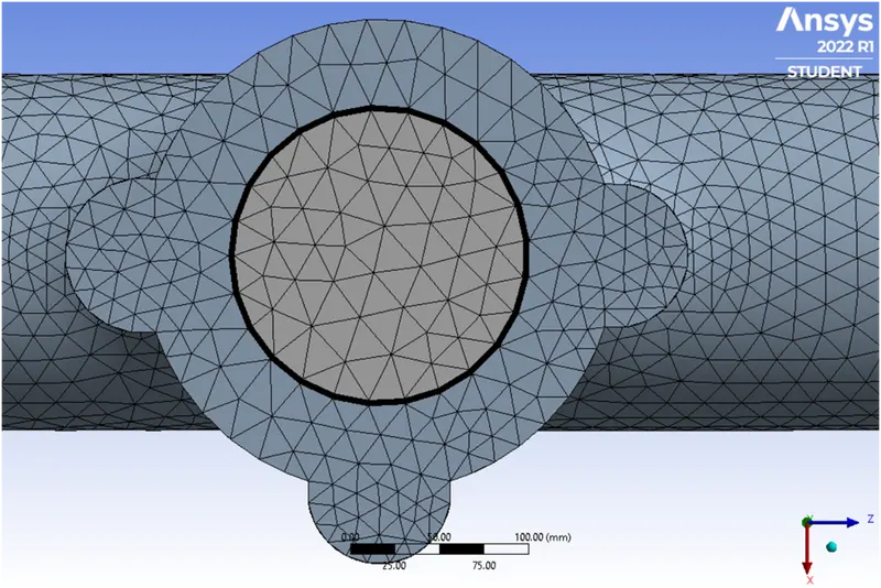
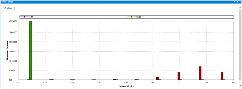
Mesh metrics

Setup

Checks mesh quality.

Solver

General

• Type – Pressure-based
• Velocity Formulation – Absolute
• Time – Steady

Reference Values

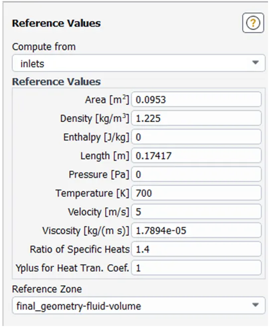
Enable energy equation

Viscous

• Turbulence
  • k-omega (2 equation)
  • Model – SST
• Material

Fluid Volume – Air

Solid Volume - Aluminum

• Boundary
  • Inlet
    • Velocity magnitude = 5 m/s
    • Temperature = 700 K
  • Outlet
    • Gauge pressure – zero Pa
  • Outer wall convection
    • Type: Wall
    • Thermal conditions – Convection

Heat transfer coefficient = 20 W/m² K

• Flanges
  • Type: Wall
  • Thermal conditions – Heat Flux

Heat Flux = 0 W/m² (Adiabatic Walls)

Solution

• Use definitions to plot-important parameters.
• Define necessary contours for tracking the result.
• Initialization using hybrid
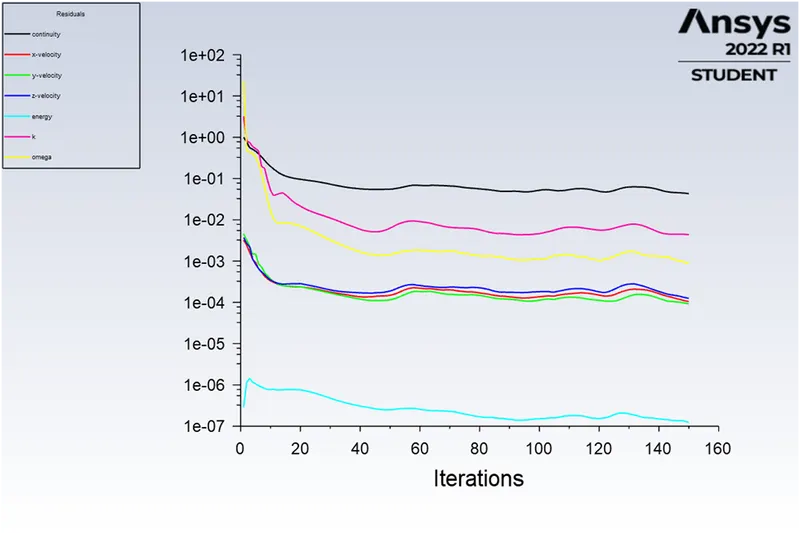
• Calculating with 150 iterations

CFD Post

After setting up the case and providing appropriate initial and boundary conditions, a number of simulations are performed on the domain. For analysis, the resulting plane can be created to view measuring parameters.

HIGHLIGHTS

Turbulence Model

K-omega SST turbulence model

• K-omega turbulence model is a common two-equation turbulence model that is used as a closure for the RANS equations. The model attempts to predict turbulence by two partial differential equations for two variables, k (turbulence kinetic energy) and ω (specific rate of dissipation of the turbulence kinetic energy k into internal thermal energy).
• SST (Menter’s shear stress transport) turbulence model is a widely used and robust two-equation eddy-viscosity turbulence model used in CFD. The model combines the k-omega turbulence model and k-epsilon turbulence model such that the k-omega is used in the inner region of the boundary layer and switches to the k-epsilon in the free shear flow.

Y+ value

• Y+ value is maintained according to the turbulence model.
• For k-omega SST turbulence model y+ value lies between 0.1 and 5.
• Considered y+ value = 1

Calculations

• Freestream velocity,u = 5 m/s
• Freestream density,ρρ = 1.225 kg/m³
• Dynamic viscosity,μμ = 1.81 * 10 ^-5 kg/m*s
• Length,L = 0.174 m
• Y+ = 1

Reynolds Number

Re = ρ⋅u⋅Lμρ⋅u⋅Lμ = 58881.215

Skin friction coefficient

C_f = (0.026)/Re^1/7 = 0.005414

Wall shear stress

ττ _wall = (C_f * ρρ * u²)/2 = 0.0829

Friction velocity

_Ufriction = (ττ_wall / ρρ)^0.5 = 0.26015

First layer thickness

∠s∠s = (y+ * μμ)/(u_friction * ρρ) = 5.695 * 10 ^-5 m = 0.06 mm

Heat Transfer Coefficient

• The analytical value of the heat transfer coefficient is 19.4287 W/m²
• The numerical result for the HTC value is 21.4798 W/m²

Nusselt Number

In fluid dynamics, the Nusselt number (Nu) is the ratio of the convective to conductive heat transfer at a boundary in a fluid.

Nu = hL/k

• h is the convective heat transfer coefficient,
• L is the characteristic length
• K is the thermal conductivity

Significance

• Nusselt number is a key parameter in determining the mode of heat transfer.
• When Nu = 1, then the amount of heat transfer by conduction and convection will be equal.
• When Nu > 1, then the amount of heat transfer by convection is more than conduction.
• When Nu < 1, then the amount of heat transfer by conduction is more than convection.

RESULT

Residual plot

Surface heat transfer coefficient plot

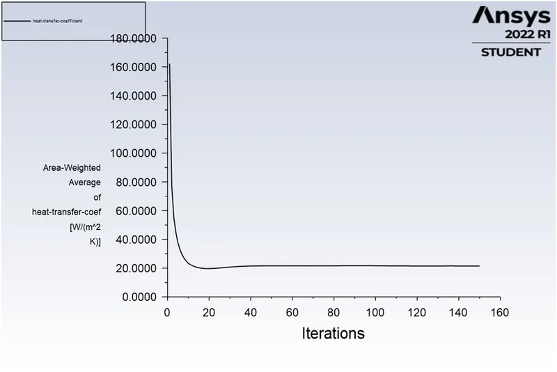
HTC value computed at outer wall convection = 21.479815

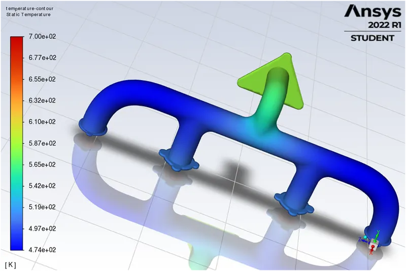
Temperature contour

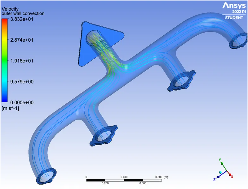
Streamline representation of velocity

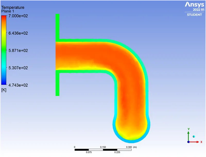
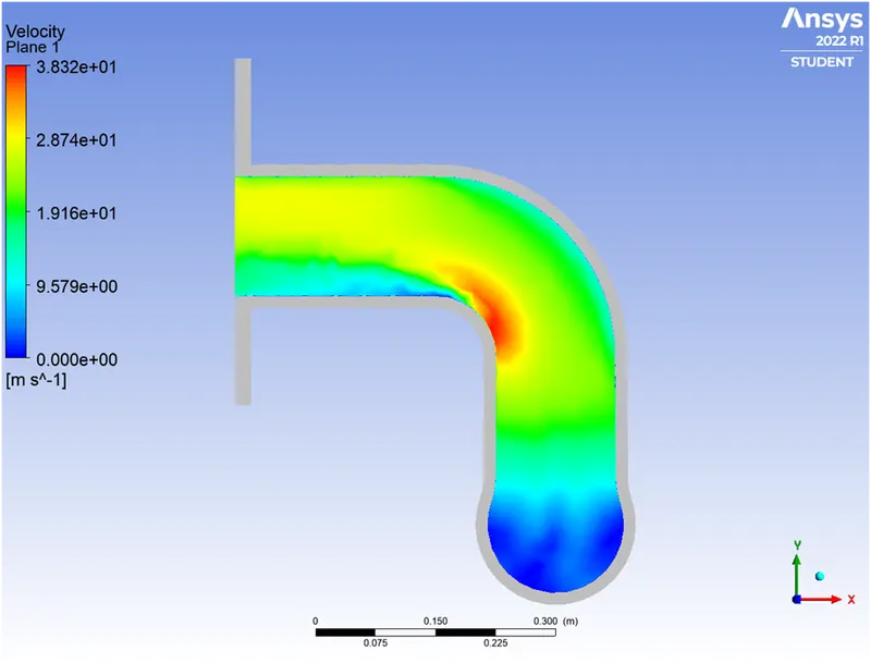
Plane showing outlet flow:

Temperature contour

Velocity contour

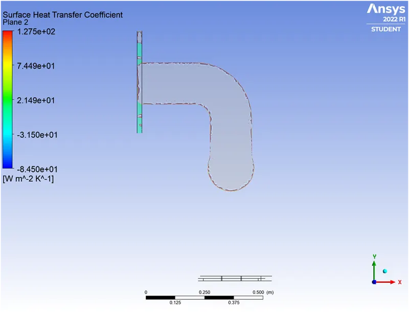
Surface HTC contour

CONCLUSION

• The CHT analysis on the exhaust port was simulated successfully on Ansys-fluent.
• The pressure-based, coupled scheme solver is used to discretize the whole geometry.
• The velocity at the outlet is higher than the velocity at the inlet shows the conservation of mass. There are four inlets against one outlet.
• The accuracy of the heat transfer coefficient depends on selecting the suitable value of y+ and turbulence model K-omega SST model. The HTC values predicted by CFD were validated against the numerical solution depicted the deviation in the range of 5% to 10% which is in compliance with industrial standards. However, the accuracy itself depends on the accuracy of the analytical solution, flow properties, and geometry. The values predicted by the baseline mesh and the refined mesh were close to each other this can be attributed to the fact that the boundary keeps on growing and declining from the inlet to the outlet owing to change in velocity, thus the value is predominant at the outlet section of the exhaust port.