Week 3 - Solving second order ODEs

SECOND ORDER ODE-SOLUTION

AIM: To solve a second order ordinary differential equation denoting the movement of a pendulum.

MAIN PROGRAM

clear all
close all
clc


t_span= [0 20];%ARRAY TO STORE THE TIME SPAN FROM 0 TO 20 SECONDS
y0=[0 5];%INITIAL BOUNDARY CONDITIONS TO STORE THE ANGULAR DISPLACEMENT AND ANGULAR VELOCITY

[t,y]=ode45('ode_func',t_span,y0);% FUNCTION TO CALCULATE THE ANGULAR DISPLACEMENT AND ANGULAR VELOCITY CALLING THE FUNCTION 'ode_func' 
disp1=y(:,1); % ARRAY TO STORE THE DISPLACEMENT VECTOR
vel=y(:,2); %ARRAY TO STORE THE VELOCITY VECTOR

figure(1)
plot(t,y(:,1))% PLOT ANGUAR DISPLACEMENT AGAINST TIME
hold on
plot(t,y(:,2))% PLOT ANGUAR VELOCITY AGAINST TIME
ylabel('ANGULAR DISPLACEMENT/ANGULAR VELOCITY')
xlabel('TIME')
hold off
legend('Angular Displacement','Angular Velocity')

figure(2)
x_0=0;%INITIALISING X BASE POINT
y_0=0;%INITIALISING Y BASE POINT

ct=1;% COUNT NUMBER

for i=1:length(disp1)

    x1= +1*sin(disp1(i,1));% CALCULATING THE VALUE OF END POSITION OF PENDULUM IN X CORDINATE
    y1=-1*cos(disp1(i,1));% CALCULATING THE VALUE OF END POSITION OF PENDULUM IN Y CORDINATE
    
    plot([x_0 x1],[y_0 y1],'color','r')% CREATING LINE CONNECTING X AND Y COORDINATE
    hold on
    plot(x_0,y_0,'s','Markersize',10)% CREATING MARKER FOR THE BASE POINT
    plot(x1,y1,'.','Markersize',50)% CREATING MARKER FOR THE BALL AT END OF PENDULUM

    axis([-2 2 -2 2])
    pause (0.1)
    hold off
    M(ct)=getframe(gcf);% COMMAND TO CAPTURE THE PLOT CREATED
    ct=ct+1; % INCREAMENTING THE COUNT VALUE BY 1
    
    

end

 movie(M)% OPEN THE ARRAY M ONCE TO DISPLAY
 videofile=VideoWriter('pendulum.avi','Uncompressed AVI'); % TEMPORARY FILE 'videofile ' TO SAVE THE FRAMES
 open(videofile)
 writeVideo(videofile,M)%WRITE THE 'videofile' WITH M ARRAY CONTAING FRAMES
 close(videofile)

FUNCTION:

function [dy_dt]= ode_func(t,y)
l=1;
m=1;
b=0.05;
g=9.81;

v=y(2);
a=-(b/m)*y(2)-(g/l)*sin(y(1));
dy_dt=[v ; a];

end

OBJECTIVE

1. Find the position and velocity of the pendulum at different time step varying from 0 to 20seconds
2. Plot the movement ofpendulum as animated graph.
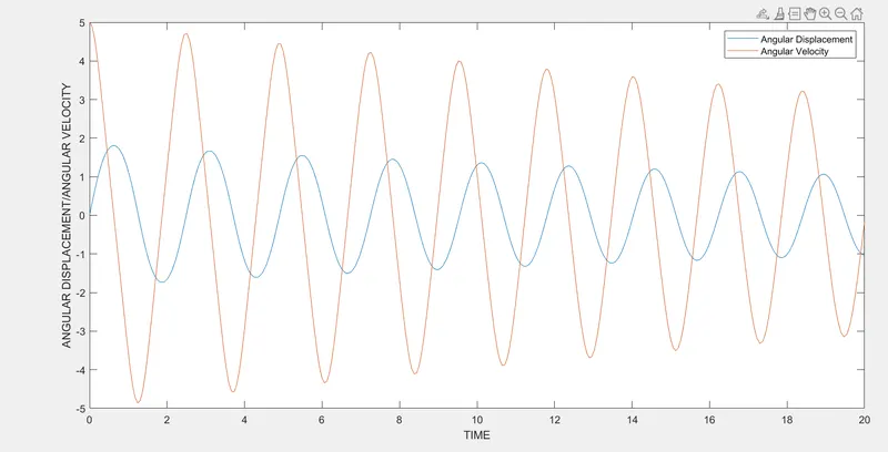
3. Plot variation of dispacement and angular velocity of pendulum against time

PRINCIPLE:

Movement of a pendulum is descibed based on ordinary differential equation as given below

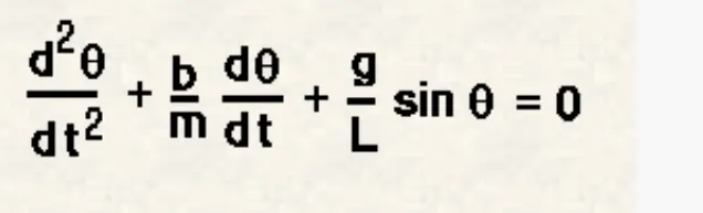
Thus objective is to find the displacement and velocity given the damping coefficient, mass of pendulum, Length of pendulum.

The given second order differentialequation is converted into two first order differential equation

These first order differential equation can be integrated to find the dispacement and velocity vector

An in-built function names ode45 is used to integrate the first order ordinary differential equation

Thus ode45 returns the displacement and angular velocity.

The displacement of pendulum over different timestep can be used to plot the aniated image

RESULTS

1. PLOT OF ANGULARDISLACEMENT/ANGULAR VLOCITY AGAINST TIME

2. ANIMATED VIDEO OF DAMPING PENDULUM

https://drive.google.com/file/d/11_Bbvs1_n_Zs8apqFhzH1k4IZorQByte/view?usp=sharing