Week-6 Calculate the Stretch Ratio by comparing the ELFORM (-2,-1,1,2) with Ogden_Material Model.

Aim- Calculate the stretch ratio by comparing the ELFORM (-2,-1,1,2) with Ogden_Material Model

Objective-

• Create a block of 10mmx10mmx10mm dimension with 10 elements for each direction and use the material card attached (Ogden_Material.k)
• Use appropriate boundary conditions to simulate tensile behavior for the model and finally compare the results from your simulation to the plot given in the question to stretch ratio 5.
• Compare the results for the simulation using ELFORM = 1, 2, -1, -2
• Use a proper solver (Implicit/Explicit) and also explain the reason.

Procedure:

1. Modeling:Modeling of the block of 10mmx10mmx10mm dimension with 10 elements for each direction was done by Mesh- shape mesher- solid box and giving the dimensions.

2. Section: The model has solid elements and we have to compare the results for the simulation using ELFORM = 1, 2, -1, -2 we change the ELFORM for every simulation in *SECTION_SOLID CARD.

EQ.-2: fully integrated S/R solid intended for elements with poor aspect ratio, accurate formulation.
EQ.-1: fully integrated S/R solid intended for elements with poor aspect ratio, efficient formulation.
EQ.1: constant stress solid element (default).
EQ.2: fully integrated S/R solid.

3. Material :The Material card attached (Ogden_Material.k) was used. It is a hyperelastic material model used to define the non linear behaviour of the materials such as rubber,polymer etc,

4. Part: Hence, the part was defined with the provided section and material .

5. Boundary conditions:

Two types of boundary conditions are implemented to simulate the tensile simulation.

1. Boundary SPC:

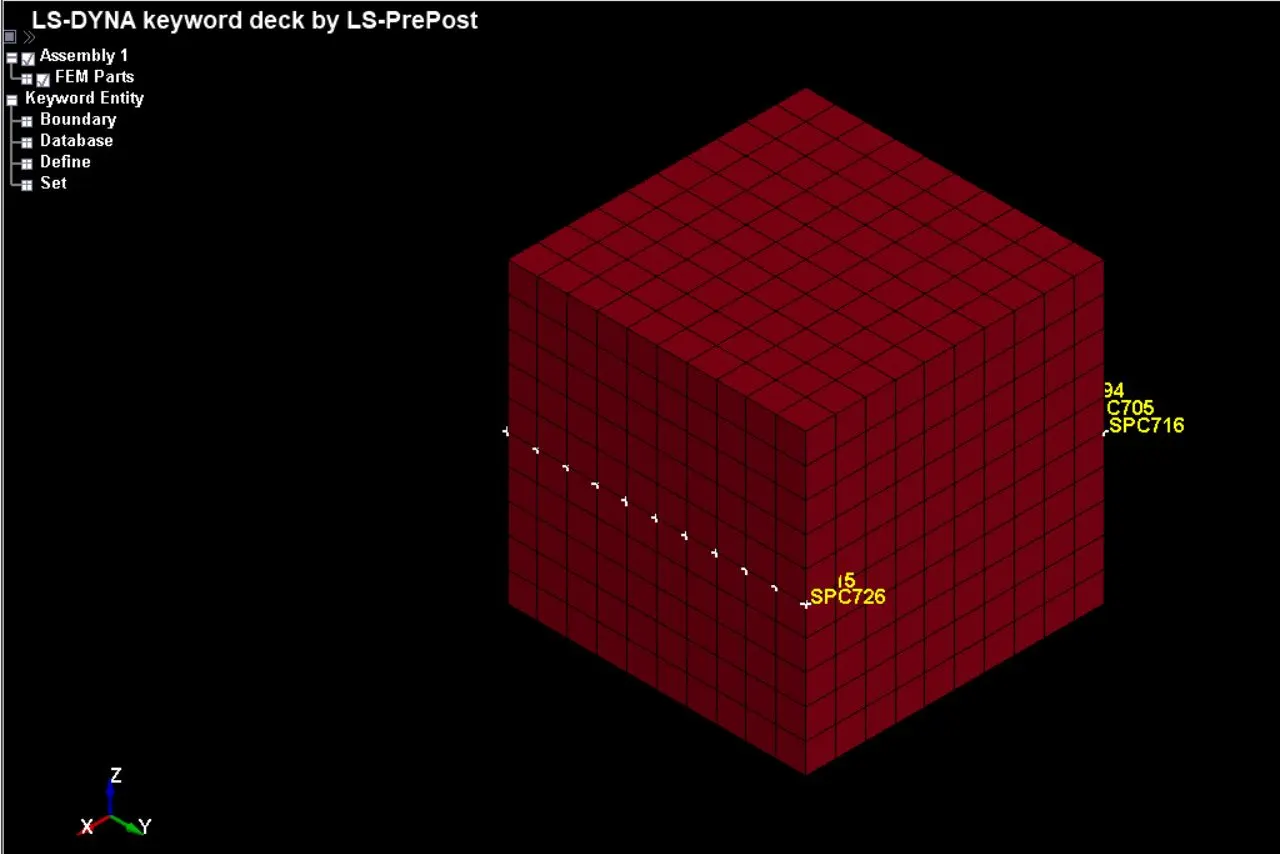
To simulate the tensile behavior, we have to make sure that one end is constrained and in the other end motion is prescribed.

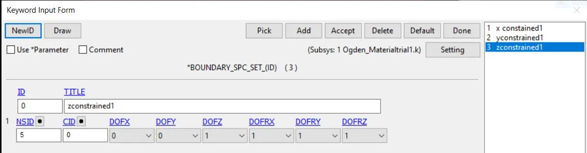
As it is a solid box, and when due to tensile load the cube elongates then the edges and other faces shrinks a bit, that are normal to the applied load and also the centre nodes ovf that face should be constrained such that they do not move. Hence we have use 3 SPC constrain cards in translational x, y and z direction as shown below.

Fig- SPCX CONSTRAINED card

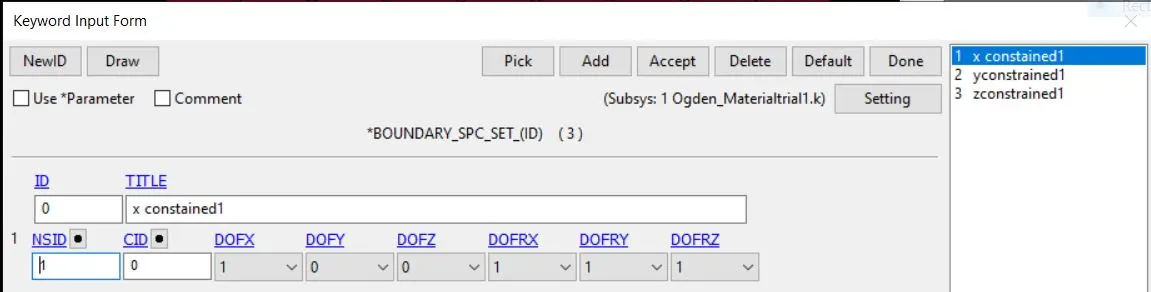
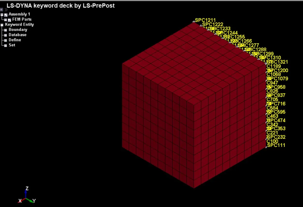
Fig- SPC Y CONSTRAINED card

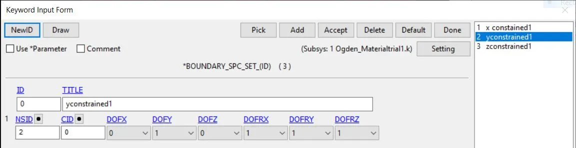
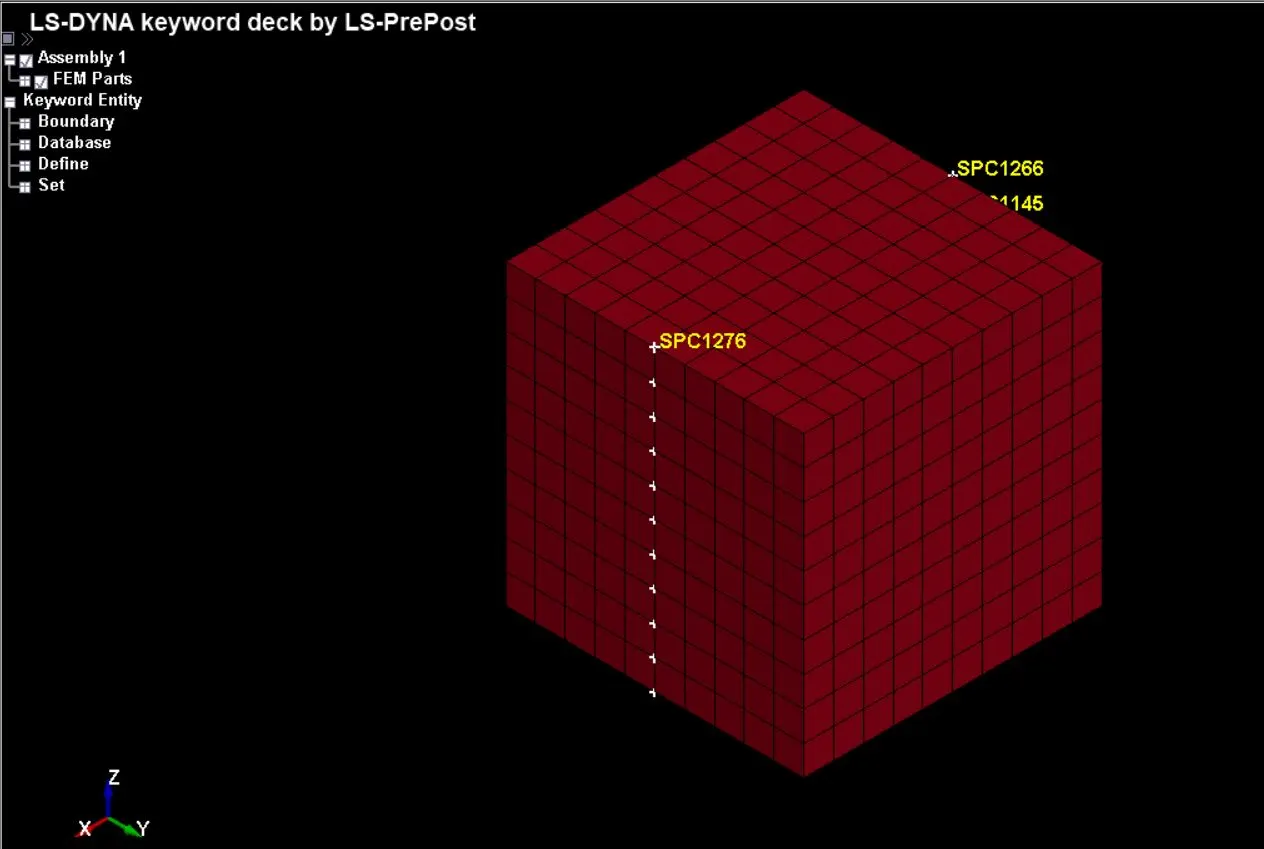
Fig- SPC Z CONSTRAINED card

2. Prescribed Boundary motion:

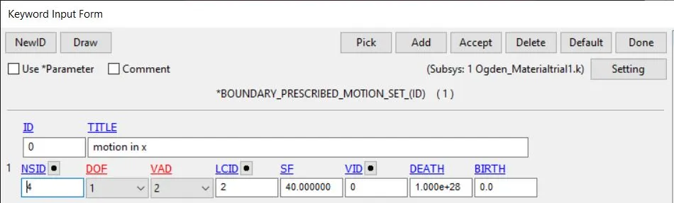
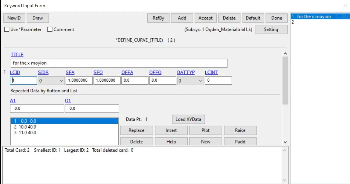
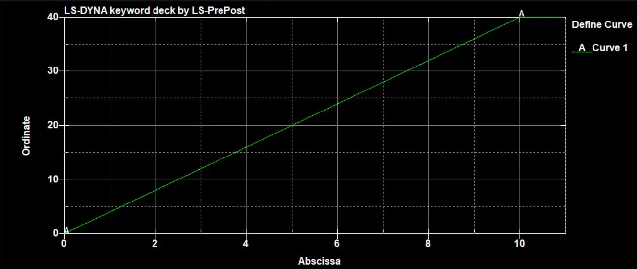
To simulate the tensile behavior , the face on the opposite side of the constrained face was to be given a displacement and as in our case we were to consider upto stretch ratio=5, Thus, we have to calculate the minimum displacement for our case.

Now, we know that,

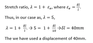
Thus a curve was defined in order to implement that as shown below.

ddd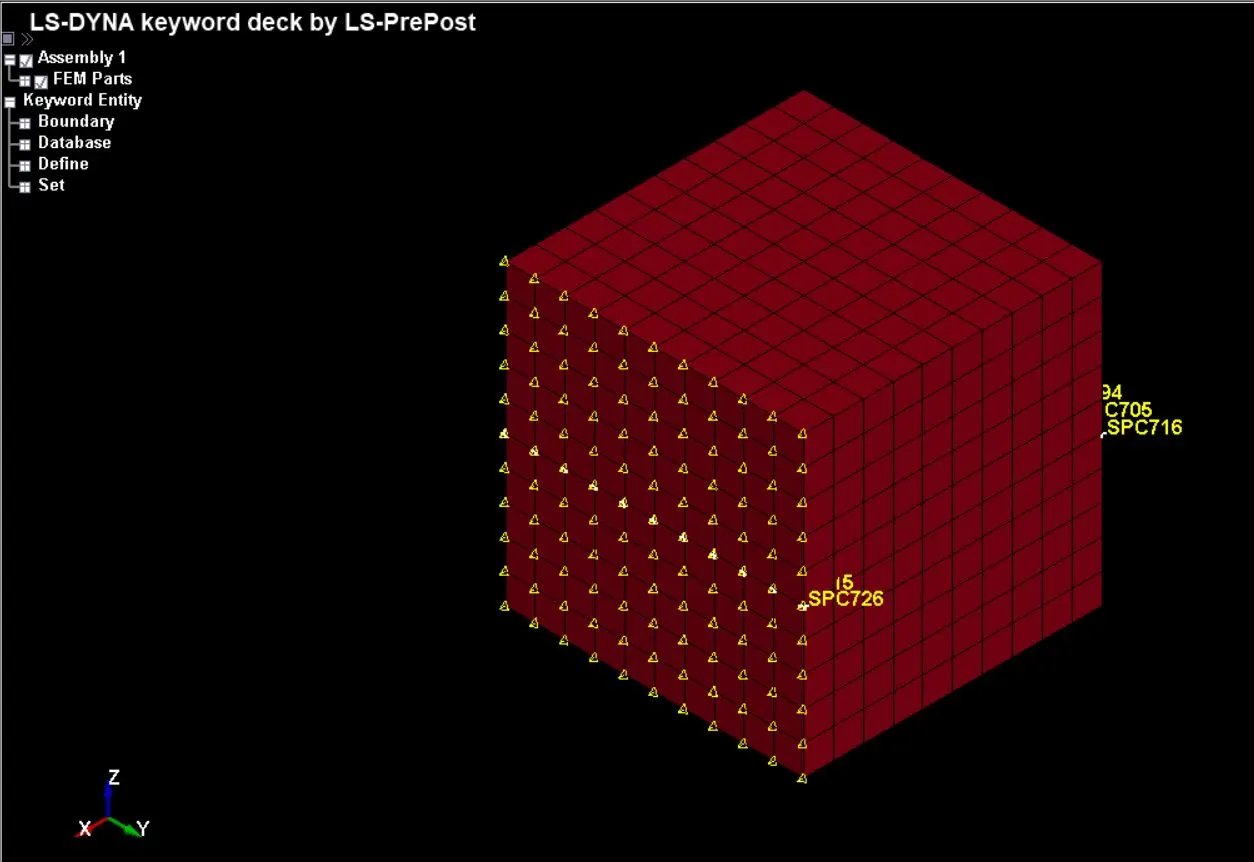Reason behind selecting an implicit solver: The material used in our case is ogden , It is a hyperelastic material model used to define the non linear behaviour of the materials. This material n on linearity is the reason the model is considered to be non linear. Also, it is a quasi static process in our case, and as it is a tensile behavior so a displacement is implemented in the form of preload.

So, in order to implement the implicit solver some important cards were used as mentioned below,

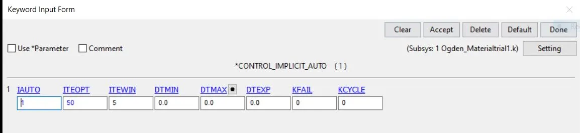
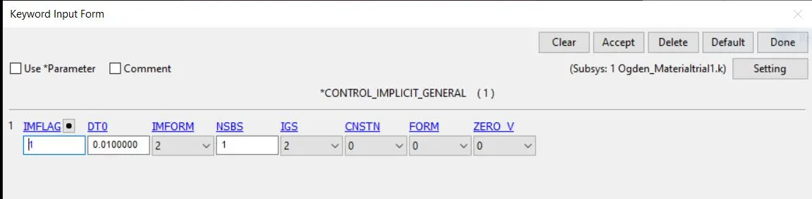Control termination card is used:

Output cards: ASCII cards of ELEOUT, Nodeout, GLSTAT was used with dt 0.01.

Database Binary D3plot of dt 0.01 was used.

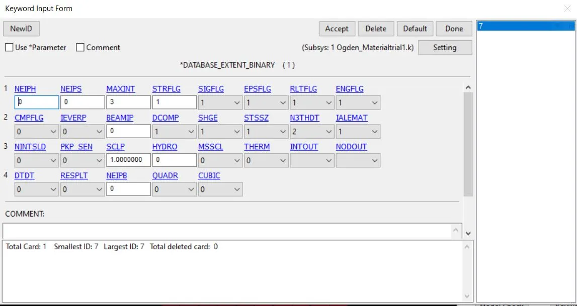
*Database_Extend_Binary card and activate the STRFLG to get the strain data.

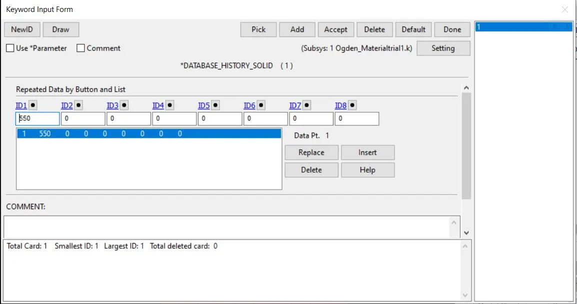
We then select element ID 550 as it is located in the center face, Database history solid card is used to get the strain values.

Post Processing:

d3HSp, d3plot was run and used for post processing and also in the post processing, we select HISTORY- ELEMENT- X stress - plot and lower ipt strainx - plot and save the curves and then using XY plot option, we select CROSS and the saved X stress and lower ipt strainx to plot the stress vs strain plot for each ELFORM simulation.

The stress and strain output of LS DYNA are true stress and true strain but we need to convert the true stress/strain value to Eng.stress/ engineering strain, and then calculate the stretch ratio.

Effective stress plot for the case of Elform 1: (Maxm and Minm value of stress are shown in the plots)

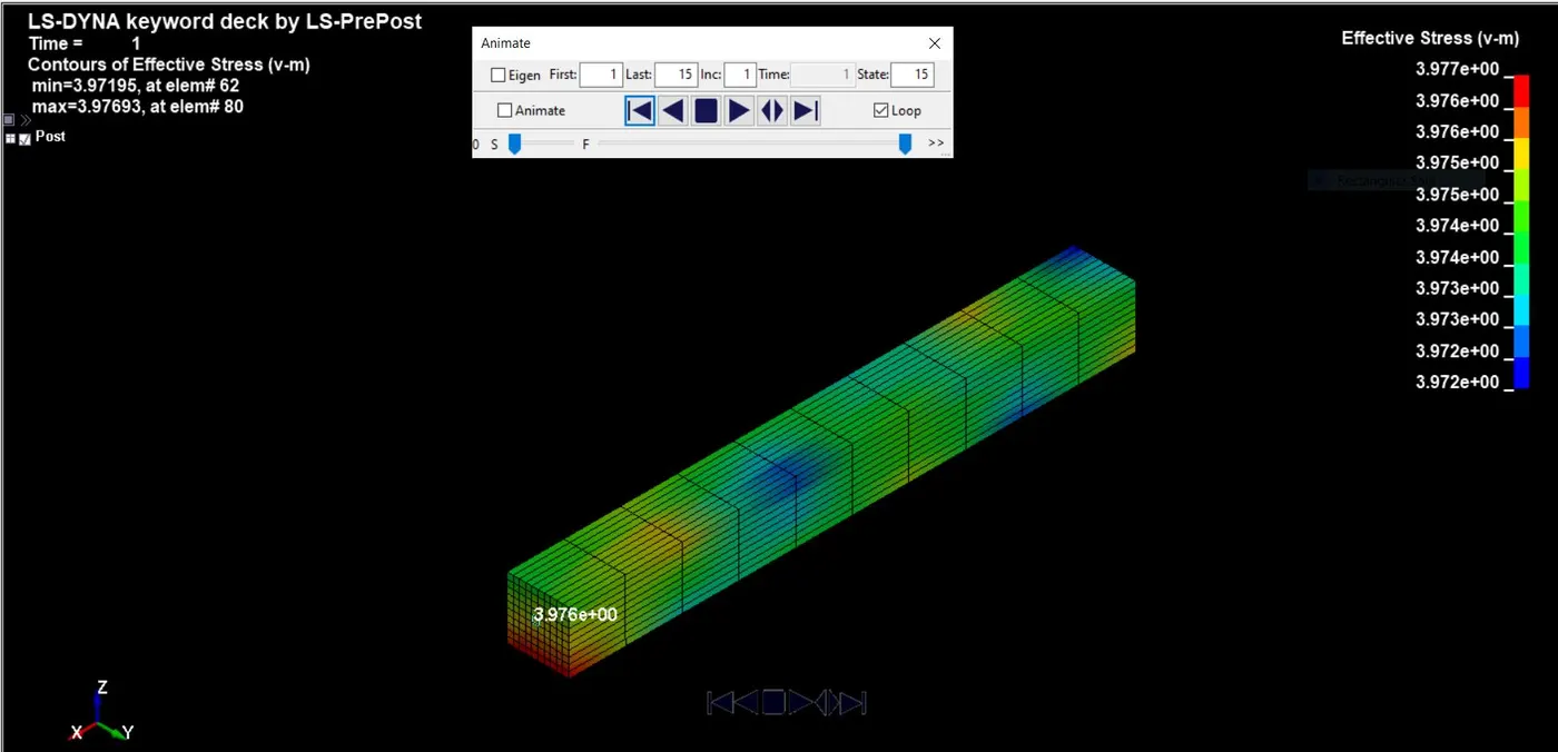
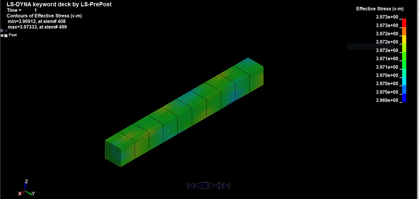
Effective stress plot for the case of Elform -1: (Maxm and Minm value of stress are shown in the plots)

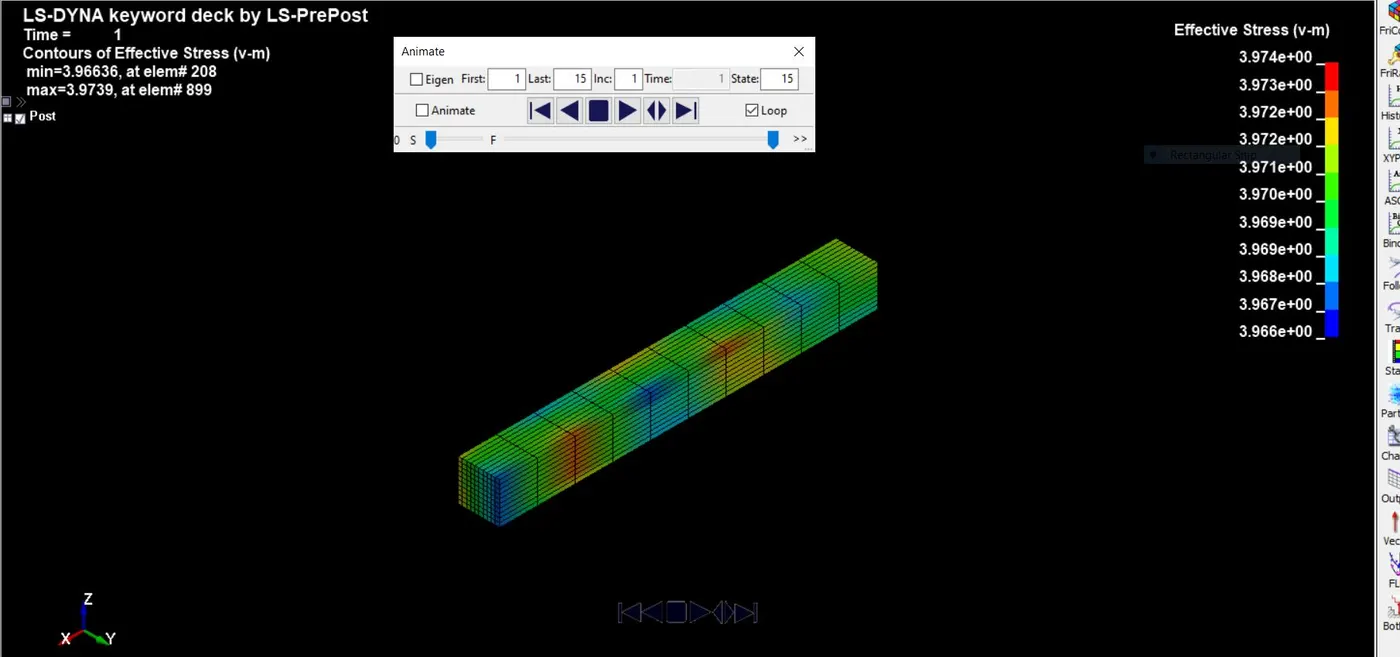Effective stress plot for the case of Elform 2: (Maxm and Minm value of stress are shown in the plots)

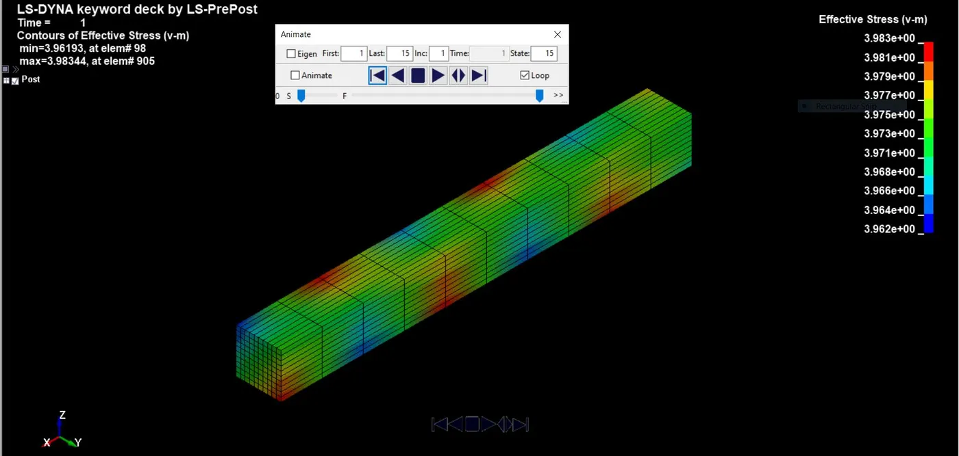Effective stress plot for the case of Elform -2: (Maxm and Minm value of stress are shown in the plots)

As explained in the formulas above, all the datas for each case were output as .csv files and Engineering Stress Vs Stretch curves for each Elform cases was plotted to compare with the uniaxial curve provided in the question, the plots were found to be sufficiently comparable. All the excel files with the relevent cases and calculations are attached with the submission.

The plots are shown below:

FIg : Engineering Stress (MPa) Vs Stretch curve for ELFORM -2

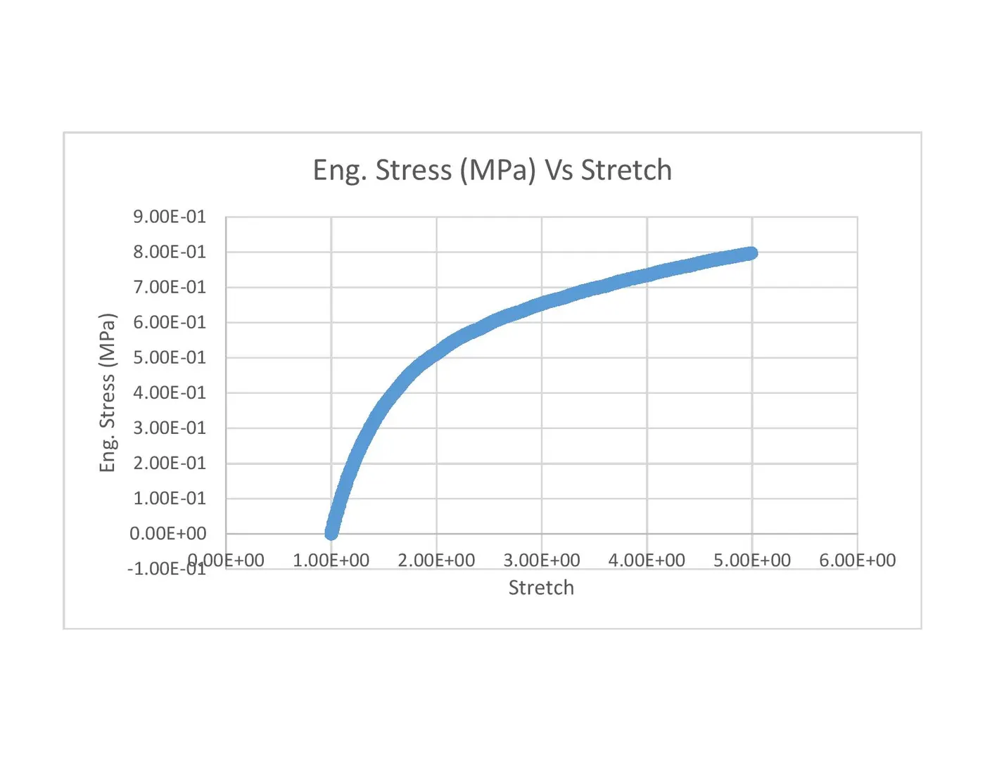
FIg : Engineering Stress (MPa) Vs Stretch curve for ELFORM -1

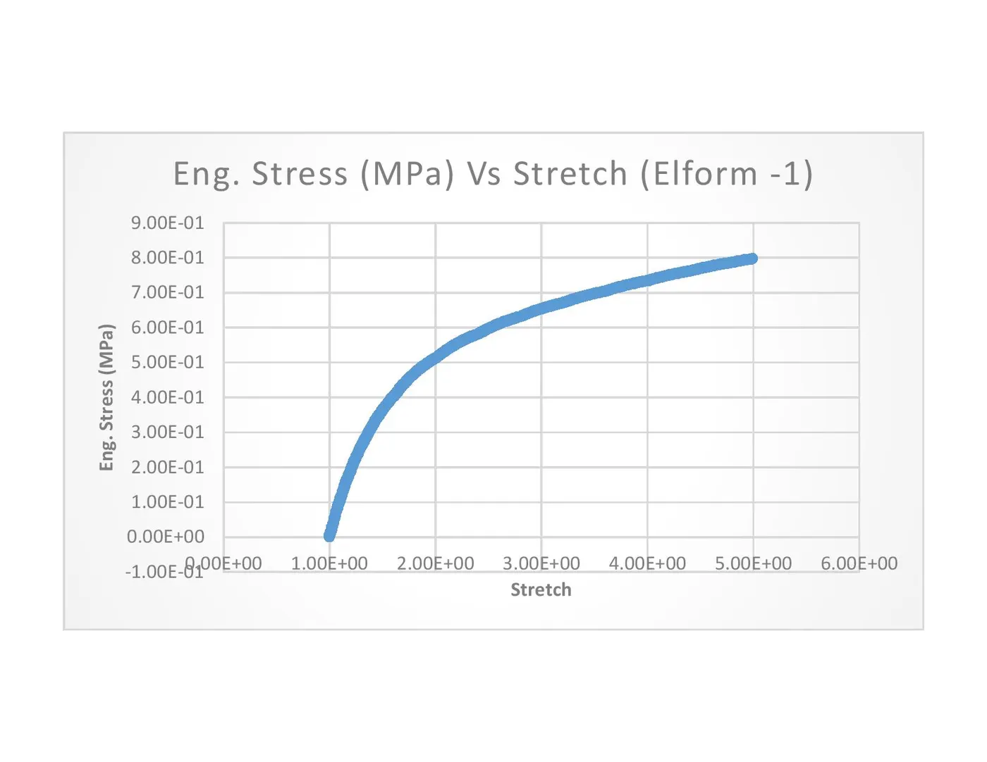
FIg : Engineering Stress (MPa) Vs Stretch curve for ELFORM 1

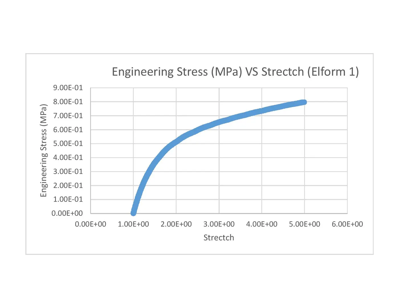
FIg : Engineering Stress (MPa) Vs Stretch curve for ELFORM 2

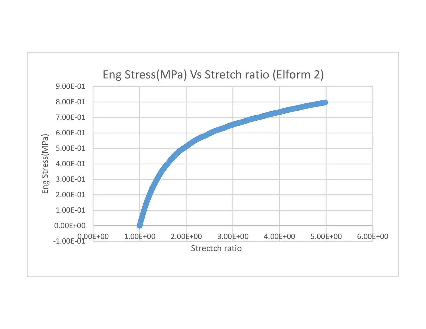Conclusion: All the Eng. Stress vs stretch ration curves of the 4 cases of ELFORM was almost similar, but in comparision with the uniaxial plot given in the question, we can see that in the question the stretch ration of 5 s obtained at the Eng. stress of about 1.8MPa, where as in our cases the same phenomanun happen within the range of (0.7-0.8) MPa range, This difference could also be attribute to the difference in the tensile testing circumstances or exact parameter differences.