Week-6 Calculate the Stretch Ratio by comparing the ELFORM (-2,-1,1,2) with Ogden_Material Model.

Comparison of stretch ratios calculated using different element formulations for a block modelled using Ogden material model.

1. Introduction

The Ogden material model is a hyperelastic material model used to describe the non-linear stress-strain behaviour of complex materials such as rubbers and biological tissue. The model relies on the fact that the material behaviour can be described by means of a strain energy density function, whence the stress-strain relationships can be derived. The Ogden model is often used to model rubber-like materials such as polymers, and biological materials. These materials can generally be considered to be isotropic, incompressible and strain rate independent.

In this exercise, a 10*10*10 mm cube was modelled with the Ogden material model available in the LS-Dyna and it was simulated for a uniaxial tensile test. Different element formulations; 1,2,-1,-2 were used one by one for the solid elements of the box and the stretch ratio was compared up to 5 as explained in the following sections.

Following hints were provided for the exercise:

• LS-DYNA the output of stress and strains from Post FringeComp Stress/Strain is given as true stress and strains.
• Stretch ratio l is defined as the ratio between the final length L and the initial length L0 of a component i.e. it is equal to (1 + engineering strain)
• Your boundary condition should be relatable to the real-time boundary condition.
• You need to add *Database_Extend_Binary card and activate the STRFLG to get the strain data.

2. The geometry:

The shape mesher tool available in the mesh tab of the LS-Pre-Post was used to model a solid box meshed with Hexa elements as shown in the attached figure.

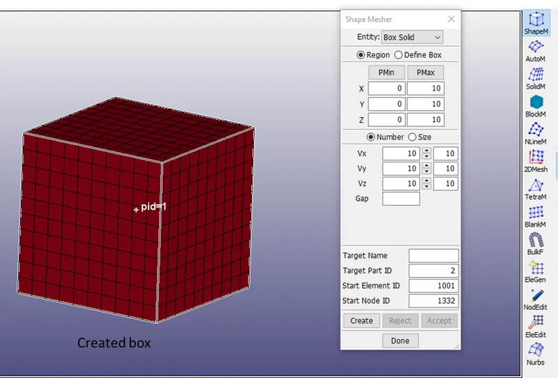
Fig 2.1: The shape mesher function used to get a meshed box of 10*10*10 mm with 10 elements in each direction

3. The material and section properties

An Ogden material card was used for modelling rubber material for the box as shown in the attached figure. The default unit used for this exercise is [gm-mm-ms].

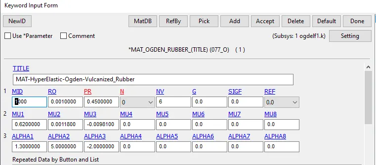
Fig 3.1: The Ogden material model used for modelling rubber

As clear from the above figure there are modulus values MU1 and MU2 apart from the usual density and Poisson's ratio.

After that, a solid section card was used for modelling the section properties of the Hexa elements. The element formulation was changed in each simulation subsequently as 1, -1, 2,-2 for the study.

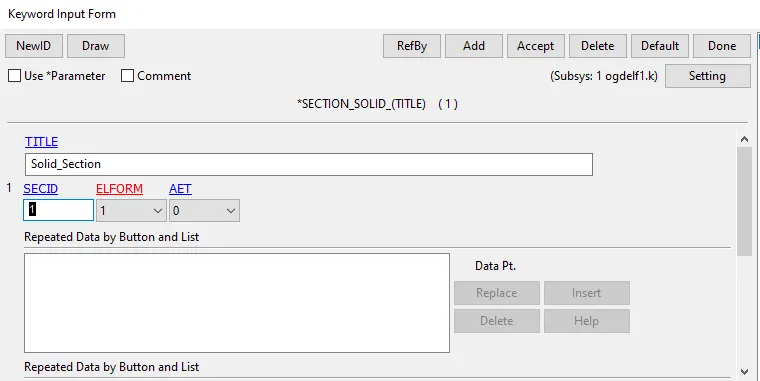
Fig 3.2: The solid section card used for the section properties of the Hexa elements.

4. Boundary conditions

A single point constraint was used to fix one face of the box. The details of the SPC constraints are shown in the attached figures.

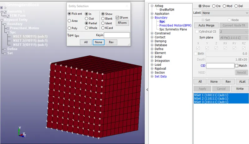
Fig 4.1: the nodes fixed for translation in the x-direction and all the rotation DOFs.

After that to simulate the gripping the nodes were constrained in Y and Z translations as shown in the attached figure:

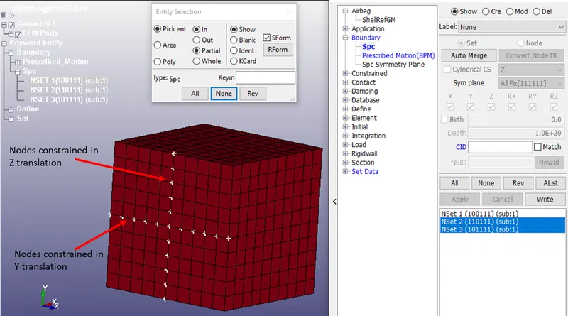
Fig 4.2: The nodes constrained in Y and Z translations respectively

After that, displacement was provided to the opposite face nodes as shown in the attached figure.

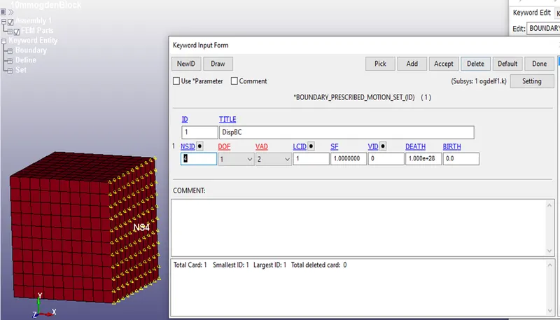
Fig 4.3: The displacement boundary applied to the node-set for translation in the X direction

A load curve was used to provide the displacement in a systematic manner. Actually, for things to work we needed deformation up to a stretch ratio of 5, so trial and error were applied and a displacement of 40 mm was applied over a time period of 2ms. The load curve is shown in the attached figure.

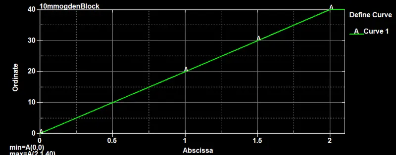
Fig 4.4: The load curve used for providing displacement boundary condition

5. Solver Settings and Control cards

This case can be simulated best using an implicit solver as the deformation involved is very large and we need to simulate it for a longer duration. In our case, it was run for 2.5 ms with an implicit scheme. Various control cards used are shown in the attached figures:

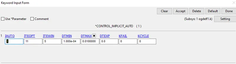
Fig 5.1: Control implicit Auto card used for the model

IAUTO was set to 1 meaning the automatic timestep adjustment was turned on. The ITEOPT and ITEWIN values were left default meaning a total of 16 iterations were allowed for a timestep and the timestep size is adjusted if the equilibrium for a step is reached 16 iterations. If it takes more than 16 iterations for residuals to fall below tolerances, the stiffness matrix is reformed. DTMIN was kept to 1e-4 which is a standard value and DT max was set to 0.01 as we're going for a DTO value of 0.001 (the thumb rule says DTmax= DT*10).

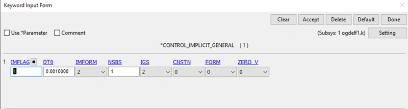
Fig 5.2: Control Implicit General card used for the model

The IMFLAG was set to 1 to indicate that the implicit solver needs to be used throughout the simulation.

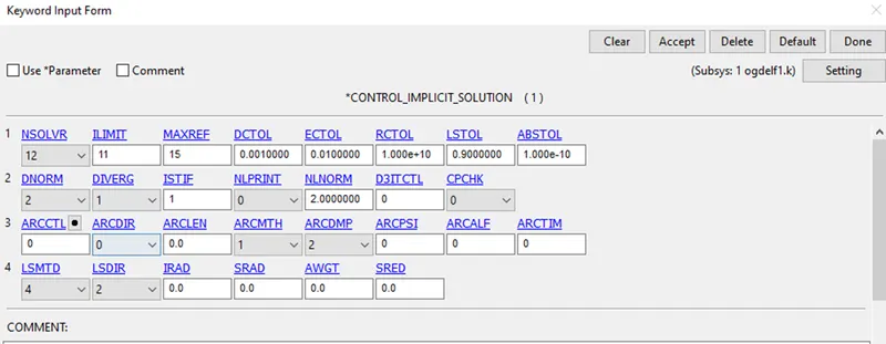
Fig 5.3: The control implicit solution card used for modelling

The DCTOL and ECTOL values were kept default as shown in the above figure. Apart from this, an implicit solver card was also used with default values for the simulation.

6. Output Requests

D3 plot, ASCI options GLSTAT, MSATSUM were used and an extent binary card was used to enable recording of the strain data.

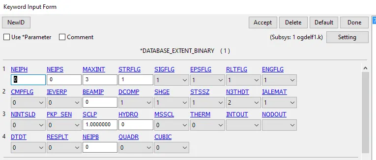
Fig 5.4: The extent binary card used in the model

The STRFLG value was set to 1 meaning we need the solver to record the strain data as well.

After this, the element identify tool was used to get the element ID of the middle element using the blank option to hide the elements. It was 546 and this value was recorded for future use while extracting the stress-strain data.

Then the simulations were run for each element formulation and results were processed using excel.

6. Results and discussion

Animation of the tensile test

``

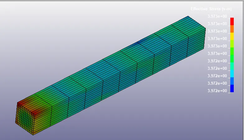
Fig 6.1: The stress contour for the elongation produced in the block

The maximum stress produced in the elements of the block was around 3.973 MPa. The stress-strain data from the LS_prepost were extracted as csv file and they were processed to get the stretch ratio using the calculations shown below:

• The values obtained from the solver are true stress and strain values.
• `sigma t=sigma e *(1+epsilon e)`
• `epsilon t = ln (1+epsilon e) = ln lambda`
• Where `sigma e`is the engineering stress, `sigma t`is the true stress, `epsilon e and epsilon t`are engineering and true strains respectively. `lambda`is the stretch defined as `(l+Delta l)/l`

6.1 Element formulation 1

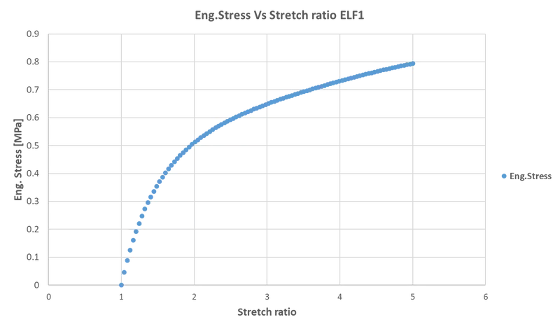
Fig 6.1.1: The Eng. stress Vs Stretch ratio graph for element formulation 1

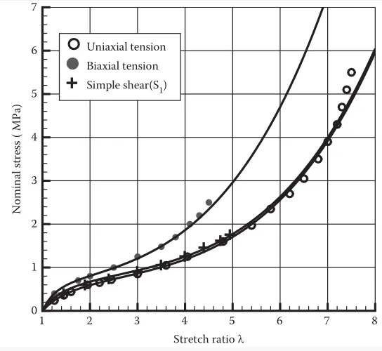
Fig 6.1.2: The comparison curve plot provided as reference.

The comparison shows the uniaxial tension curve misses the shape after stretch ratio 2 and this miss can be attributed to a number of facts like inaccuracy in the FE model and different loading cases.

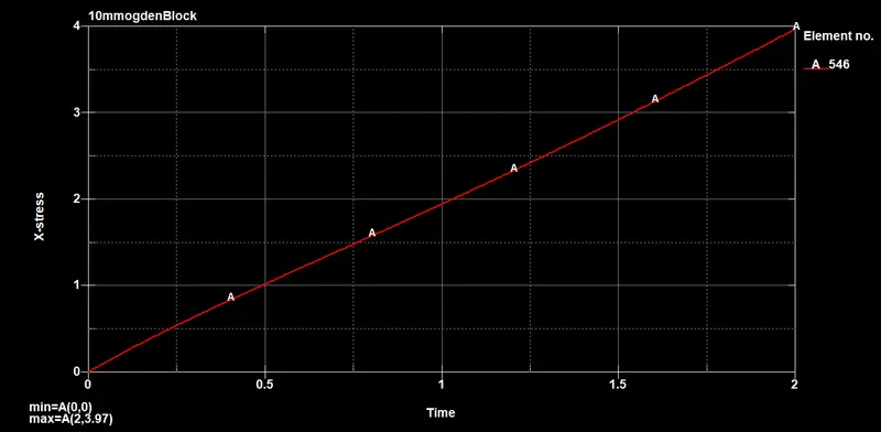
Fig 6.1.3: The stress curve for the element 546

The max stress obtained is in agreement with the data shown by the stress contour in fig 6.1.

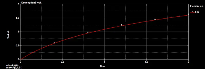
Fig 6.1.4: The Strain curve obtained for the element 546

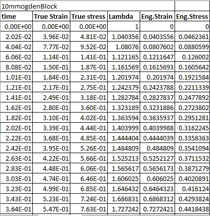
Fig 6.1.5: The snapshot of excel sheet used for calculations

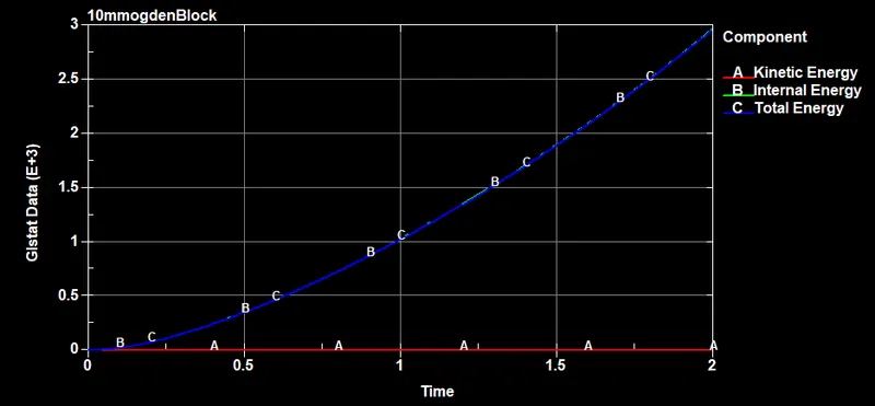
Fig 6.1.6: the different energies

It is evident that as the work is being done on the specimen, its internal energy is rising, so is the total energy which in in accordance with the conservation law.

6.2 The element formulation 2

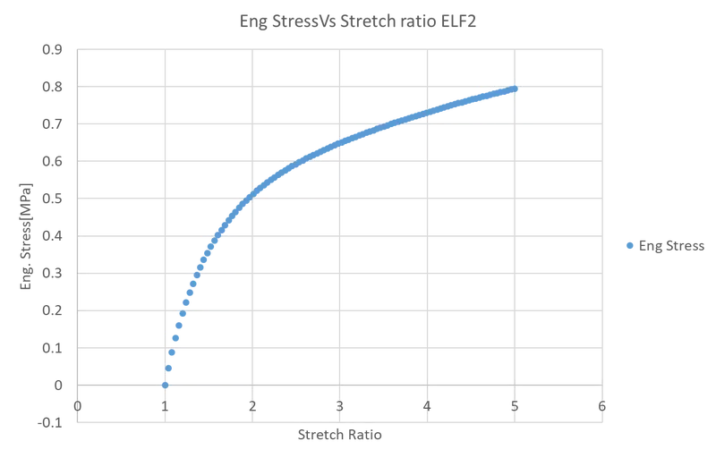
Fig 6.2.1: The Eng. stress Vs Stretch ratio graph for element formulation 2

Again the shape is more or less same and no visible difference can be observed.

6.3 The element formulations -1 and -2

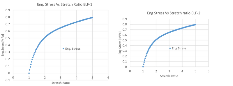
Fig 6.3.1: The Eng. stress Vs Stretch ratio graph for element formulation -1 and -2.

Slight deviation of stress value in the elf -1 can be observed at the bottom and elf -2 looks the same in comparison to elfs 1 and 2.

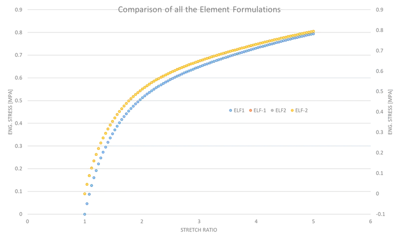
Fig 6.3.2: The comparison of different ELFs

Slight deviations can be observed among the different ELFs which is expected and no solid comment can be passed based on this exercise as it was intended just for making familiar with the implicit solver settings in the LS-Dyna.